Global mean surface temperature projection

Last update: 26 September 2017

suppressPackageStartupMessages(library(INLA))
suppressPackageStartupMessages(library(tidyverse))
knitr::opts_chunk$set(
  cache.path='_knitr_cache/global-temperature/',
  fig.path='figure/global-temperature/'
)

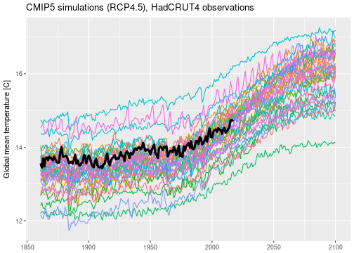
CMIP5 (“Coupled Model Intercomparison Project”) is a coordinated climate modeling experiments set up by climate centers around the world to compare their climate model results. Data from the CMIP5 runs can be downloaded by researchers for free after asking for permission. For this project, I looked at annually and globally averaged surface temperatures simulated by 35 different climate models. All models were run from 1860 to 2100 under emission scenario RCP4.5 (RCP stands for “representative concentration pathway”) which is considered a moderate, neither overly optimistic nor pessimistic, trajectory of future green house gas emissions.

I have also downloaded observed global mean temperatures from the HadCRUT4 data set. These historical temperature reconstructions come as a collection of 100 ensemble members to estimate observational uncertainty. I simply took the 100 member median and ignored the uncertainty information provided, effectively treating the observations as perfect. The observed global mean temperatures are currently available for 1860 to 2017.

Below is a plot of the entire data set.

plot of chunk plot-cmip5-data

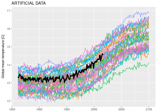
I’m not sure whether or not I’m allowed to publish the raw CMIP5 data here, which means that I am probably not. So I simulated some artificial data to work with that looks similar to the real CMIP5 global temperature projections. You can find the simulation code in the repository, file global-temperature.Rmd, code block simulate-data.

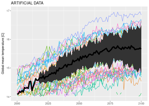
The simulated data is saved in the data directory. Here is the psychedelic spaghetti plot:

load('data/gmst_sim.Rdata')
ggplot() + 
  geom_line(data=gmst_mod_sim, aes(x=year, y=gmst, color=model)) + 
  geom_line(data=gmst_obs_sim, aes(x=year, y=gmst), lwd=1.5, na.rm=TRUE) +
  theme(legend.position = 'none') +
  labs(x=NULL, y='Global mean temperature [C]', color=NULL) + 
  ggtitle('ARTIFICIAL DATA')

plot of chunk plot-simulated-data

The goal is to use all the data, the climate model simulations and the historical observations of the real world (black line) to predict the future evolution of the real world. There are a few difficulties though.

Most models do not reproduce past climate very well. The simulated historical temperatures range from 12 to 14 degrees which constitutes a significant range around the relatively stable 13.25 degrees measured in the real world up to 1950. Should we discard those models that can’t replicate past climate? Or does the fact that all model runs increase over time tell us something about the real world? Given that all those models have hard climate science and decades of expertise behind them, we should be wary to throw any data away.

We should not interpret the range of simulated temperatures in 2100 as “the uncertainty range” about future climate. If we did this, we would also have to interpret the simulated temperature range for next year (2018) as “the uncertainty range” for 2018. This is obviously nonsense to think that next years temperature is likely to be between 13.5 and 15.5 degrees, if the biggest year-to-year increment we have ever observed is on the order of 0.2 degrees. Temperature projections of the near future should be close to the last recorded temperature value, because this is how the climate system seems to behave given everything we know. So uncertainty ranges in the near future should be narrower than for the far future, and all projections should be constrained by the historical observations.

How do we use all the available information, while avoiding these pitfalls? Enter the Rougier et al (2013) framework.

The co-exchangeable framework

Rougier et al (2013) published an inferential framework for a collection of climate model runs that are judged to be exchangeable, i.e. no climate model is a priori different from the others, and a real world climate that is co-exchangeable with the model climates, i.e. no climate model is a priori better at representing the real world than any other. Under some constraints on how beliefs are expressed statistically, the co-exchangeable collection of model runs and their relationship to the real world are expressed by the following statistical model.

Climate model runs $X_1, …, X_m$, each of which can be a high-dimensional vector containing simulation of past and future climate, is represented as the sum of a common mean $M$ and mutually independent, zero-mean residuals $R_i$:

\begin{equation} X_{i,t} = M_t + R_{i,t} \end{equation}

The real world climate, which is co-exchangeable with the model runs, is expressed in terms of the common mean $M$ by

\begin{equation} Y_{t} = A M_t + U_{t} \end{equation}

where $A$ is a constant matrix (set to $1$ in the original paper), and $U$ is the discrepancy. The historical observations $Z$ are noisy, incomplete measurements of the real world climate, represented through the incidence matrix $H$ and zero-mean, independent measurement error $W$:

\begin{equation} Z = H Y + W \end{equation}

The challenge is to model the random components $M$, $R$, and $U$.

For simplicity I will make a very strong assumptions, namely that real climate is exchangeable with model climates. This implies that $E[U] = 0$ and $var(U) = var(R)$. In that case $U$ and $R$ are independent samples from the same distribution, and with the additional choice $A = 1$, $Y$ behaves statistically just like the $X_i$.

With 35 model runs, the common mean component $M$ can be estimated with high precision. I will model $M$ simply by a random walk

\begin{equation} M_{t+1} = M_t + \Delta_t \end{equation}

with constant, but unknown variance of the increments $var(\Delta_t)$.

The individual residuals $R_i$ will be modeled as the sum of three random terms:

a systematic bias term, constant over time, different for each model
a stationary AR1 process, to account for internal variability around the common mean which exhibits auto-correlation
a non-stationary random walk with small variance of the increments, to account for the fact that model climates can drift away slowly from the common mean.

\begin{equation} R_{i,t} = B_i + U_{i,t} + V_{i,t} \end{equation}

where

\begin{align} U_{i,t+1} & = \alpha U_{i,t} + \sigma \epsilon_{i,t} \newline V_{i,t+1} & = V_{i,t} + \tau \epsilon’_{i,t} \end{align}

R-INLA

We want to use INLA to decompose the data into a common mean and independent residuals. A crucial feature is the replicate option in INLAs f() function for which the package documentation currently says

replicate: We need to write documentation here

There is a short paragraph at r-inla.org on how replicate is used. If you specify, say, an AR1 model by f(i, model='ar1', ...) and provide i = c(1,2,3,1,2,3) in your data, INLA will assume that the first triplet of data values and the second triplet of data values depend on the exact same realisation of the latent AR1 process. If you additionally set replicate = c(1,1,1,2,2,2) in the model definition, INLA will model the first and second triplet as 2 independent realisations of the latent AR1 process. We make use of this feature when distinguishing between common and individual terms in the model definition. We have to set the correct indices i and correct values for replicate.

inla_formula = gmst ~ 
                 -1 + 
                 f(i1, model='rw1') +                  
                 f(i2, model='iid', replicate=repl) +  
                 f(i3, model='ar1', replicate=repl) + 
                 f(i4, model='rw1', replicate=repl, 
                       prior='loggamma', param=c(25, .25))

where i1 to i4 and repl are defined in the data specification:

inla_data = 
  gmst_mod_sim %>%
  bind_rows(
    gmst_obs_sim %>% 
    bind_rows(data_frame(year=2018:2100, gmst=NA_real_)) %>%
    mutate(model = 'obs')
  ) %>%
  mutate(i1 = year) %>%
  mutate(i2 = 1L) %>%
  mutate(i3 = year) %>%
  mutate(i4 = year) %>%
  mutate(repl = as.integer(as.factor(model)))

print(inla_data)

## # A tibble: 8,640 x 8
##        model  year     gmst    i1    i2    i3    i4  repl
##        <chr> <int>    <dbl> <int> <int> <int> <int> <int>
##  1 ACCESS1-0  1861 13.14903  1861     1  1861  1861     1
##  2 ACCESS1-0  1862 13.09299  1862     1  1862  1862     1
##  3 ACCESS1-0  1863 13.21700  1863     1  1863  1863     1
##  4 ACCESS1-0  1864 13.23755  1864     1  1864  1864     1
##  5 ACCESS1-0  1865 13.07631  1865     1  1865  1865     1
##  6 ACCESS1-0  1866 12.88249  1866     1  1866  1866     1
##  7 ACCESS1-0  1867 12.85828  1867     1  1867  1867     1
##  8 ACCESS1-0  1868 12.96236  1868     1  1868  1868     1
##  9 ACCESS1-0  1869 13.01687  1869     1  1869  1869     1
## 10 ACCESS1-0  1870 12.92496  1870     1  1870  1870     1
## # ... with 8,630 more rows

The first bind_rows directive adds NAs to the observations for the years 2018-2100. These are interpreted as missing values so INLA will fill them in, which will be used as our temperature predictions. Then we append the observed temperatures to the simulated temperatures. Then we specify the time indices i1 to i4 as documented below. We set repl = as.integer(as.factor(model)), so each model is assigned a unique, constant number. Using replicate = repl, each model will be treated as an independent realisation of the respective process.

Our INLA formula has the following components:

f(i1): Random walk process, indices are 1:n for each model (and for the observations). No replication is set, i.e. each model and the observation sees the same realisation of the random walk process. This is the common mean $M$.
f(i2): iid process. The time indices are constant, but each model sees an independent realisation because replicate is set. This is the model specific constant offset $B_i$.
f(i3): AR1 process, with time indices 1:n for each model, with replicate set. Each model sees an independent realisation of an AR1 process with the same parameters.
f(i4): As for i3, but using a random walk process. This models non-stationary behavior of the residuals due to model simulations “drifting away” from the common mean.

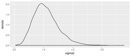
I found that when using the default prior specifications for the random walk process f(i4) I got error messages due to stability issues, possibly because the “common random walk plus individual random walk” model is not identifiable. I therefore put a $Gamma(25, .25)$ prior on the random walk precision (specified in INLA as loggamma prior on log-precision), which encodes my prior belief that the “drift” of the residuals is not going to be massive. I don’t expect the temperature residuals to drift much more than 1 degree per century. The $Gamma(25, .25)$ prior on the random walk precision translates into a prior on the 100-year variance of the random walk process with mode at one and mass concentrated between .5 and 1.5:

df = data_frame(sigma2 = 100 * 1 / rgamma(1e4, shape=25, rate=.25))
ggplot(df) + geom_density(aes(x=sigma2))

plot of chunk plot-rw-variance-prior

We can now fire up INLA. We tell INLA that our observations are “perfect” via family='gaussian' and using a very high precision. We also set config=TRUE to be able to simulate from the posterior later on.

inla_result = inla(formula=inla_formula, data=inla_data, family='gaussian', 
              control.family=list(initial=12, fixed=TRUE),
              control.compute=list(config=TRUE))

The code takes about a minute to run on my laptop, so for this problem INLA does not feel as lightning fast as it is often advertised. On the other hand, inferring this model using MCMC would probably take hours.

Now we sample from the posteriors, using the function inla.posterior.sample(). I am not 100 percent sure what is going on under the hood of this function. For example, I don’t know what algorithm is used to draw the samples. The help file isn’t terribly enlightening. But after looking at the results further down I think it is doing something reasonable.

set.seed(23)
inla_sampls = inla.posterior.sample(n=100, result=inla_result, seed=42) 

The output is a list of length 100 (number of samples). Each sample creates a list with elements hyperpar, latent, and logdens. We are interested in the latent samples, as these also contain samples named Predictor. In fact there are 8640 Predictor samples:

inla_sampls[[1]][['latent']] %>% str

##  num [1:26196, 1] 13.2 13.1 13.2 13.2 13.1 ...
##  - attr(*, "dimnames")=List of 2
##   ..$ : chr [1:26196] "Predictor:0001" "Predictor:0002" "Predictor:0003" "Predictor:0004" ...
##   ..$ : chr "sample1"

inla_sampls[[1]][['latent']] %>% rownames %>% grep(x=., 'Predictor', value=TRUE) %>% range

## [1] "Predictor:0001" "Predictor:8640"

Since 8640 is the length of the model plus observation data frame, I am guessing that the predictors map to the rows of the inla_data data frame. So we have to find those predictors that correspond to model == obs. This is what the following chunk of code does. The output of inla.sample.posterior is not “tidy”, so there is a bit of data wrangling necessary.

obs_inds = paste('Predictor:', which(inla_data$model == 'obs'), sep='')
obs_sampls = 
  inla_sampls %>%          # inla_sampls is a list of length 'number of samples'
    map('latent') %>%      # extract latents
    map(drop) %>%          # 1 column matrix to vector
    map(`[`, obs_inds) %>% # extract correct indices
    map(setNames, nm=levels(as.factor(inla_data$year))) %>% # set names to year
    map_df(enframe, .id='sample', name='year') %>%          # to long data frame 
    mutate_if(is.character, as.integer) %>%
    rename(gmst = value)

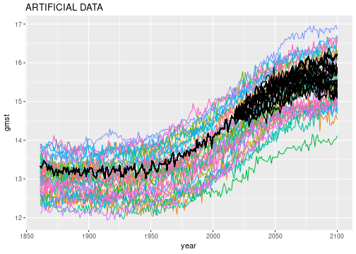
The posterior sample data is now ready to be plotted:

ggplot() +
  geom_line(data=gmst_mod_sim, aes(x=year, y=gmst, color=model)) +
  geom_line(data=obs_sampls, aes(x=year, y=gmst, group=sample), color='black') +
  theme(legend.position = 'none') +
  ggtitle('ARTIFICIAL DATA')

plot of chunk plot-inla-projection

Let’s also plot the posterior mean plus/minus 2 posterior standard deviations:

post_df = obs_sampls %>%
  group_by(year) %>%
  summarise(post_mean = mean(gmst), post_sd = sd(gmst)) %>%
  mutate(lwr = post_mean - 2 * post_sd, upr = post_mean + 2 * post_sd)

ggplot(data=post_df, aes(x=year)) +
  geom_line(data=gmst_mod_sim, aes(y=gmst, color=model), na.rm=TRUE) +
  geom_ribbon(aes(ymin=lwr, ymax=upr)) +
  geom_line(aes(y=post_mean), lwd=2, na.rm=TRUE) +
  theme(legend.position = 'none') +
  ylim(14, 17) + xlim(2000, 2100) +
  labs(x=NULL, y='Global mean temperature [C]') +
  ggtitle('ARTIFICIAL DATA')

plot of chunk plot-posterior-mean-variance

All this looks rather well. However, on closer inspection, something doesn’t seem quite right with the sampling algorithm. There are a couple of “bundles” of posterior predictive samples, which indicates that the sampler doesn’t produce independent posterior samples. Below I zoomed in on a region of the posterior predictive samples where the issue is particularly obvious:

ggplot() +
  geom_line(data=gmst_mod_sim, aes(x=year, y=gmst, color=model), na.rm=TRUE) +
  geom_line(data=obs_sampls, aes(x=year, y=gmst, group=sample), color='black', na.rm=TRUE) +
  coord_cartesian(xlim=c(2015, 2030), ylim=c(14.4, 15.0)) +
  theme(legend.position = 'none') + labs(x=NULL, y=NULL)

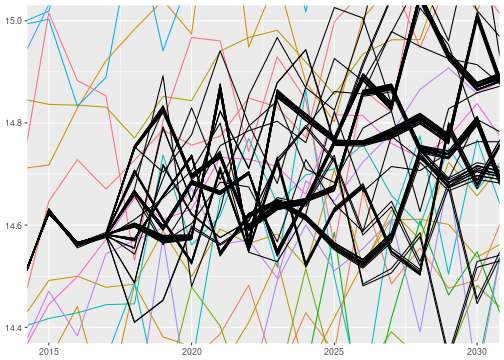
plot of chunk plot-inla-projection-bundles

I will ignore this issue for now, but it is certainly important and worthwhile looking into. It might be possible to solve this by setting some parameters to control the sampler.

The real world

I have applied the same analysis to the actual CMIP5 data and produced equivalent plots.

plot of chunk plot-inla-cmip5

plot of chunk plot-inla-cmip5-mean-var

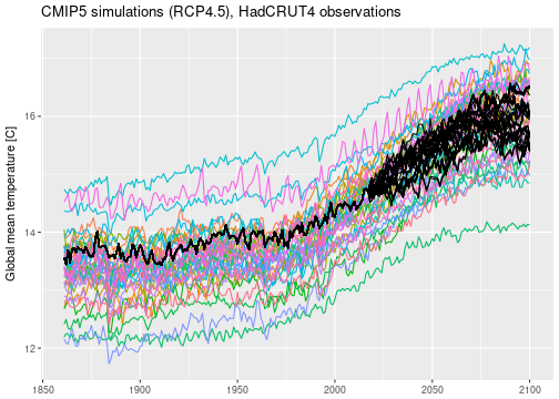
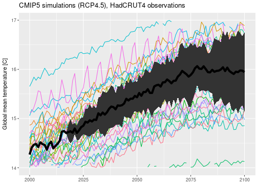
According to this analysis, we should expect an increase in global mean temperatures from pre-industrial $\approx 13.5$, currently $\approx 14.5$, to roughly between $15$ and almost $17$ degrees by the end of the century. This is a warming of $1-3$ degrees compared to the commonly used reference period 1961-1990. Remember that this is assuming that emission scenario RCP4.5 is the correct one. This result is in line with the well-known global temperature projections published for example in the IPCC summary for policymakers (Table SPM.2).

Conclusion

INLA provides a flexible modelling framework for modelling time series data. We used INLA to model a collection of exchangeable model simulations of global mean surface temperature. By treating the real-world observations as a partly observed realisation from the same exchangeable collection, we were able to predict the future by making INLA fill in the missing future values. However, the sampling algorithm used by INLA seems suboptimal, as it doesn’t produce independent posterior samples.

As an extension we could think about explicitly modelling the discrepancy between observations and ensemble mean by specifying, say, an additional random walk f(i5, model='rw1') where i5 is NA for models and 1:n for the observations. I should also include information about observational uncertainty, which is available in the HadCRUT4 archive.