Linear regression on a spatial grid
We address a commonly encountered problem in weather and climate forecasting: A data set of past atmospheric model forecasts and corresponding observations is available for a few years and many grid points. We want to use this data set to learn something about systematic errors of the forecast model, and how to correct them for future forecasts. Correcting systematic forecast errors is often done by fitting a linear regression model to the observations, that uses the model forecast as a predictor. We expect systematic errors to be different for different locations, so in principle we should fit a regression model separately at each grid point. But then atmospheric data is smooth, so we would also expect the regression parameters to vary smoothly in space.
In this note I develop a method to efficiently fit linear regression models to gridded data, while accounting for spatial smoothness of the parameter estimates. The method results in improved out-of-sample performance of the regression model.
suppressPackageStartupMessages(library(rnaturalearth))
suppressPackageStartupMessages(library(maps))
suppressPackageStartupMessages(library(tidyverse))
suppressPackageStartupMessages(library(Matrix))
suppressPackageStartupMessages(library(viridis))
knitr::opts_chunk$set(
  cache.path='_knitr_cache/grid-regression/',
  fig.path='figure/grid-regression/'
)
borders = ne_countries(scale=110, continent='Europe') %>% map_data
The data
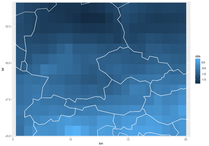
Our data set consists of climate model forecasts and corresponding observations of surface temperature over a region in central Europe in summer (June-August). There are 17 years’ worth of forecasts and observations (1993-2009) with one forecast per grid point per year. The climate model forecast were initialised in early May of the same year, so the forecast lead time is on seasonal time scales. The forecast and observation data were normalised to have mean zero and variance one.
load('data/grid-regression.Rdata') # available in the repository

# grid parameters
N_i = t2m %>% distinct(lat) %>% nrow
N_j = t2m %>% distinct(lon) %>% nrow
N_t = t2m %>% distinct(year) %>% nrow
N_s   = N_i * N_j

# lat/lon range
lat_range = t2m %>% select(lat) %>% range
lon_range = t2m %>% select(lon) %>% range

# prepare the temperature data frame
t2m = t2m %>%
  spread('type', 'temp') %>%
  mutate(i = as.numeric(factor(lat, labels=1:N_i))) %>%
  mutate(j = as.numeric(factor(lon, labels=1:N_j))) %>%
  mutate(s = (j-1) * N_i + i)

t2m
## # A tibble: 4,641 x 8
##     year   lat   lon       fcst         obs     i     j     s
##    <int> <dbl> <dbl>      <dbl>       <dbl> <dbl> <dbl> <dbl>
##  1     1 45.35  5.62 -0.5723529 -0.65581699     1     1     1
##  2     1 45.35  6.33 -0.5403007 -0.28856209     1     2    14
##  3     1 45.35  7.03 -0.4745686 -0.08392157     1     3    27
##  4     1 45.35  7.73 -0.5454510 -0.12503268     1     4    40
##  5     1 45.35  8.44 -0.6720850 -0.16267974     1     5    53
##  6     1 45.35  9.14 -0.6268562 -0.03320261     1     6    66
##  7     1 45.35  9.84 -0.5265686  0.27477124     1     7    79
##  8     1 45.35 10.55 -0.5040850  0.35745098     1     8    92
##  9     1 45.35 11.25 -0.4779935  0.11647059     1     9   105
## 10     1 45.35 11.95 -0.4878824 -0.06941176     1    10   118
## # ... with 4,631 more rows
Below we plot the observations at year $t=1$ for illustration.
ggplot(t2m %>% filter(year==1)) +
  geom_raster(aes(x=lon, y=lat, fill=obs)) +
  coord_cartesian(xlim = lon_range, ylim=lat_range) +
  geom_path(data=borders, aes(x=long, y=lat, group=group), col='white')
Linear regression on a grid
We have data on a grid with spatial gridpoints $(i,j)$, with row indices $i=1,…,N_i$ and column indices $j=1,…,N_j$. For mathematical treatment, data on 2-d grids are collapsed into 1-d vectors by stacking the grid columns, so that the grid point with coordinates $i,j$ corresponds to the vector element $s = (j-1)N_i + i$.
At each grid point $s=1,…,N_s$ and each time $t=1,…,N_t$ we have an observable $y_{s,t}$ and a covariate $f_{s,t}$ which are related by a linear function plus a random error:
\begin{equation} y_{s,t} = \alpha_s + \beta_s f_{s,t} + \sqrt{e^{\tau_s}} \epsilon_{s,t} \end{equation}
Specifically for our application we have
- $y_{s,t}$ is the observation of real climate at grid point $s$ at time $t$
- $f_{s,t}$ is the (imperfect) climate forecast for gridpoint $s$ for time $t$ that is corrected (“post-processed”) by linear regression
- $\alpha_s$, $\beta_s$ and $\tau_s$ are local parameters of the regression model, that are assumed to be constant in time but variable in space
- the residuals $\epsilon_{s,t}$ are iid standard Normal variates
Our goal is to model the regression parameters $\alpha_s$, $\beta_s$ and $\tau_s$ as being spatially smooth. Thereby the linear regression model at point $(i,j)$ can benefit from data at neighboring grid points. We should hope that borrowing strength from neigboring data, and the resulting reduction in estimator variance, improves the overall performance of the regression model.
For spatial modelling, we collect the regression parameters in the vector $x = (\alpha_1, …, \alpha_{N_s}, \beta_1, …, \beta_{N_s}, \tau_1, …, \tau_{N_s})$, which will be called the latent field.
The joint log-likelihood of the observations, given the latent field $x$ and any hyperparameters $\theta$ is proportional to
\begin{align} & \log p(y_{1,1},…y_{N_t,{N_s}} \vert x,\theta)\newline & = \sum_{s,t} \log p(y_{s,t} \vert x,\theta)\newline & \propto -\frac{N_t}{2} \sum_s \tau_s - \frac12 \sum_{s=1}^{N_s} e^{-\tau_s} \sum_{t=1}^{N_t} (y_{s,t} - \alpha_s - \beta_s f_{s,t})^2 \end{align}
The latent field $x$ is assumed to be a Gauss-Markov random field (GMRF), i.e. $x$ has a multivariate Normal distribution with zero mean vector and sparse precision matrix $Q$. We assume that the three sub-vectors of $x$, i.e. $\alpha$, $\beta$ and $\tau$, are independent, and that the precision matrices that characterise their spatial structure are $Q_\alpha$, $Q_\beta$ and $Q_\tau$. The latent field $x$ thus has distribution
\begin{align} \log p(x \vert \theta) & = \log p(\alpha \vert \theta) + \log p(\beta \vert \theta) + \log p(\tau \vert \theta)\newline & \propto \frac12 (\log\det Q_\alpha + \log\det Q_\beta + \log\det Q_\tau) - \frac12 \left[ \alpha’ Q_\alpha \alpha + \beta’ Q_\beta \beta + \tau’ Q_\tau \tau \right]\newline & =: \frac12 \log\det Q - \frac12 x’Qx \end{align}
and so $x$ is a GMRF with precision matrix given by the block-diagonal matrix $Q = diag(Q_\alpha, Q_\beta, Q_\tau)$.
The precision matrix will be specified below, but first we look at the standard method of fitting individual regression models, ignoring spatial dependency.
Linear regression without spatial dependency
We fit a linear regression model to each grid point individually without considering any smoothness of the regression parameters over neighboring grid points.
We simply use lm to fit linear models at each grid point:
# fit linear models
t2m_lm = t2m %>% nest(-c(s,lat,lon)) %>%
  mutate(fit = purrr::map(data, ~ lm(obs ~ fcst, data=.)))

# extract residuals and fitted values
t2m_lm_fit =
  t2m_lm %>%
  mutate(fit = purrr::map(fit, fortify)) %>%
  unnest(fit, data) %>%
  select(-c(.sigma, .cooksd, .stdresid)) %>%
  mutate(resid_loo = .resid / (1 - .hat)) %>%
  rename(resid = .resid,
         fitted=.fitted)

# calculate mean squared errors of raw forecasts and fitted values
t2m_lm_mse = t2m_lm_fit %>%
  summarise(mse = mean(resid^2),
            mse_loo = mean(resid_loo^2))

# output
t2m_lm_mse %>% knitr::kable()
| mse | mse_loo |
|---|---|
| 0.6612585 | 0.8995776 |
Spatial dependency
To model spatial dependency of the regression parameters, we will use a 2d random walk model, i.e. the value at grid point $(i,j)$ is given by the average of its neighbors plus independent Gaussian noise with constant variance $\sigma^2$:
\begin{equation} x_{i,j} \sim N\left[\frac14 (x_{i-1,j} + x_{i+1,j} + x_{i,j-1} + x_{i,j+1}), \sigma^2 \right] \end{equation}
This model implies that the vector $x$ is multivariate Normal with a sparse precision matrix. Note that the variance $\sigma^2$ is the only hyperparameter in this model, i.e. $\theta = \sigma^2$.
TODO: derive matrix $D$ for this model as in Rue and Held (2005, ch. 3), then $Q=D’D$, discuss free boundary conditions, and zero eigenvalues
# diagonals of the circular matrix D
diags = list(rep(1,N_s),
rep(-.25, N_s-1),
rep(-.25, (N_j-1)*N_i))
# missing values outside the boundary are set equal to the value on the
# boundary, i.e. values on the edges have 1/4 of themselves subtracted and
# values on the corners have 1/2 of themselves subtracted
edges = sort(unique(c(1:N_i, seq(N_i, N_s, N_i), seq(N_i+1, N_s, N_i), (N_s-N_i+1):N_s)))
corners = c(1, N_i, N_s-N_i+1, N_s)
diags[[1]][edges] = 0.75
diags[[1]][corners] = 0.5
# values on first and last row have zero contribution from i-1 and i+1
diags[[2]][seq(N_i, N_s-1, N_i)] = 0
# construct band matrix D and calculate Q
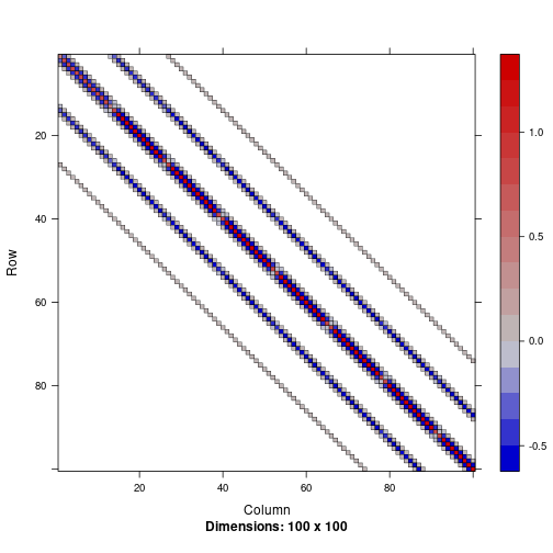
Dmat = bandSparse(n = N_s, k=c(0,1,N_i), diagonals=diags, symmetric=TRUE)
Q_alpha = Q_beta = Q_tau = crossprod(Dmat)
Below we plot a part of the precision matrix $Q$ to illustrate its structure and highlight its sparsity:
image(Q_alpha[1:100, 1:100])
Approximating $p(x \vert y, \theta)$ by the Laplace approximation
We want to calculate the posterior distribution of all the regression parameters $\alpha$, $\beta$, $\tau$ collected in the latent field vector $x$, given the observed data $y$ and specific values of $\theta$. To this end we have to normalise the joint distribution $p(y,x, \theta)$ with respect to $x$, i.e. we have to calculate the integral of $p(y,x,\theta)$ with respect to $x$, where $p(y,x,\theta)$ is given by
\begin{align} \log p(y,x) & \propto \log p(y \vert x, \theta) + \log p(x \vert \theta) + \log p(\theta)\newline & \propto -\frac{N_t}{2} \sum_s \tau_s - \frac12 \sum_{s=1}^{N_s} \sum_{t=1}^{N_t} e^{-\tau_s} (y_{s,t} - \alpha_s - \beta_s f_{s,t})^2 + \frac12 \log\det Q - \frac12 x’Qx + \log p(\theta) \end{align}
Note that the precision matrix $Q$ depends on the hyperparameter $\theta = \sigma^2$. Define the function $f(x)$ as being proportional to $\log p(y,x,\theta)$ at fixed values of $y$ and $\theta$:
\begin{equation} f(x) = - \frac12 x’Qx - \frac{N_t}{2} \sum_s \tau_s - \frac12 \sum_{s=1}^{N_s} \sum_{t=1}^{N_t} e^{-\tau_s} (y_{s,t} - \alpha_s - \beta_s f_{s,t})^2 \end{equation}
Since $f(x) \propto \log p(x \vert y, \theta)$, the mode of $f(x)$ is equal to the posterior mode of $x$ given $y$ and $\theta$. To calculate the maximum of $f(x)$ numerically, the Newton-Raphson algorithm can be used:
- an initial guess $x_0$ for the mode is proposed
- the function $f(x)$ is Taylor-expanded to second order around $x_0$
- $f(x) \approx \tilde{f}(x) = f(x_0) + (x - x_0)^\prime grad f(x_0) + \frac12 (x-x_0)^\prime Hf(x_0) (x-x_0)$ where $grad f$ is the gradient of $f$ and $Hf$ is the Hessian matrix of $f$
- the mode of the second order approximation $\tilde{f}(x)$ is given by the solution to the equation $Hf(x_0) (x - x_0) = -grad f(x_0)$ and represents as an improved estimate for the true mode of $f(x)$
- a new Taylor approximation around the new estimate $x_0$ yields a new estimate of the mode, and so the algorithm can be iterated to convergence to find the mode of $f(x)$, and thus the posterior mode of $x$ given $y$ and $\theta$
Once the estimate of the mode $x_0$ has converged, the gradient $grad f(x_0)$ is zero, and so the second order approximation of $f(x)$ is proportional to $\tilde{f}(x) \propto -\frac12 (x-x_0)^\prime [-Hf(x_0)] (x-x_0)$. Since $f(x)$ is proportional to $\log p(x \vert y, \theta)$, the second order approximation of $f(x)$ that $p(x \vert y, \theta)$ is approximated by a Gaussian with mean $x_0$ and precision matrix $-Hf(x_0)$.
Laplace approximation: $p(x \vert y, \theta)$ is approximated by a Gaussian with mean equal to the mode of $f(x)$ (which is found numerically), and precision matrix given by the negative Hessian of $f(x)$ evaluated at the mode.
The gradient of $f(x)$ is a vector of length $3 N_s$, comprised of the three gradient vectors $(\partial_\alpha f, \partial_\beta f, \partial_\tau f)$, given by
\begin{align} \frac{\partial f}{\partial \alpha} & = -Q_\alpha \alpha + vec_s\left[ e^{-\tau_s} \sum_t (y_{s,t}-\alpha_s-\beta_s f_{s,t}) \right]\newline \frac{\partial f}{\partial \beta} & = -Q_\beta \beta + vec_s\left[ e^{-\tau_s} \sum_t f_{s,t}(y_{s,t}-\alpha_s-\beta_s f_{s,t}) \right]\newline \frac{\partial f}{\partial \tau} & = -Q_\tau \tau + vec_s\left[ \frac12 e^{-\tau_s} \sum_t (y_{s,t}-\alpha_s-\beta_s f_{s,t})^2 -\frac{N_t}{2} \right] \end{align}
The Hessian of $f(x)$ is the block matrix
\begin{equation} Hf(x) = \left(\begin{matrix} H_{\alpha\alpha}-Q_\alpha & H_{\alpha\beta} & H_{\alpha\tau}\newline H_{\alpha\beta} & H_{\beta\beta} -Q_\beta& H_{\beta\tau}\newline H_{\alpha\tau} & H_{\beta\tau} & H_{\tau\tau} -Q_\tau \end{matrix}\right) \end{equation}
with diagonal matrices of second derivatives given by
\begin{align} H_{\alpha\alpha} & = diag_s \left[ - N_t e^{-\tau_s} \right] \newline H_{\alpha\beta} & = diag_s \left[ - e^{-\tau_s} \sum_t f_{s,t} \right] \newline H_{\alpha\tau} & = diag_s \left[ -e^{-\tau_s} \sum_t (y_{s,t} - \alpha_s - \beta_s f_{s,t}) \right] \newline H_{\beta\beta} & = diag_s \left[ -e^{-\tau_s} \sum_t f_{s,t}^2 \right] \newline H_{\beta\tau} & = diag_s \left[ -e^{-\tau_s} \sum_t f_{s,t} (y_{s,t} - \alpha_s - \beta_s f_{s,t}) \right] \newline H_{\tau\tau} & = diag_s \left[ -\frac12 e^{-\tau_s} \sum_t (y_{s,t} - \alpha_s - \beta_s f_{s,t})^2 \right] \end{align}
The function calc_f below returns a list with the value of $f$, the gradient $grad f$ and the Hessian matrix $Hf$ at a given value of $x$:
calc_f = function(x, sigma2, data) {
# function that returns a list of f, grad f, hess f as function of sigma2 (the
# innovation variance of the 2d random walk)
# data is a data frame with columns: s, year, obs, fcst

  N_s = data %>% distinct(s) %>% nrow
  N_t = data %>% distinct(year) %>% nrow

  alpha = x[1:N_s]
  beta = x[1:N_s + N_s]
  tau = x[1:N_s + 2*N_s]
  df_x = data_frame(s = 1:N_s, alpha=alpha, beta=beta, tau=tau)
  df = data %>%
    # join alpha, beta, tau to data frame
    left_join(df_x, by='s') %>%
    # add fitted values and residuals
    mutate(yhat = alpha + beta * fcst,
           resid = obs - yhat) %>%
    # calculate the necessary summary measures for gradient and hessian
    group_by(s) %>%
    summarise(
      tau         = tau[1],
      exp_m_tau   = exp(-tau),
      sum_resid   = sum(resid),
      sum_resid_2 = sum(resid ^ 2),
      sum_f_resid = sum(fcst * resid),
      sum_f_2     = sum(fcst ^ 2),
      sum_f       = sum(fcst))


  derivs = df %>% mutate(
             dgda   = exp_m_tau * sum_resid,
             dgdb   = exp_m_tau * sum_f_resid,
             dgdt   = -N_t/2 + 0.5 * exp_m_tau * sum_resid_2,
             d2gdaa = -N_t * exp_m_tau,
             d2gdbb = -exp_m_tau * sum_f_2,
             d2gdtt = -0.5 * exp_m_tau * sum_resid_2,
             d2gdab = -exp_m_tau * sum_f,
             d2gdat = -exp_m_tau * sum_resid,
             d2gdbt = -exp_m_tau * sum_f_resid) %>%
           arrange(s)

  # calculate f(x)
  f = with(df, -N_t/2 * sum(tau) - 0.5 * sum(exp_m_tau * sum_resid_2)) -
        0.5 * drop(crossprod(alpha, Q_alpha) %*% alpha +
                   crossprod(beta,  Q_beta)  %*% beta  +
                   crossprod(tau,   Q_tau)   %*% tau) / sigma2

  # the gradient
  grad_f = c(-drop(Q_alpha %*% alpha) / sigma2 + derivs$dgda,
             -drop(Q_beta  %*% beta)  / sigma2 + derivs$dgdb,
             -drop(Q_tau   %*% tau)   / sigma2 + derivs$dgdt)

  # the hessian
  hess_f =
    - bdiag(Q_alpha, Q_beta, Q_tau) / sigma2 +
    with(derivs, bandSparse(
      n = 3 * N_s,
      k = c(0, N_s, 2 * N_s),
      diagonals= list(c(d2gdaa, d2gdbb, d2gdtt), c(d2gdab, d2gdbt), d2gdat),
      symmetric=TRUE))

  return(list(f=f, grad_f=grad_f, hess_f=hess_f))

}
The function calc_x0 uses the derivatives returned by calc_f to iteratively find the mode of $f(x)$, and thus the mode of $p(x \vert y, \theta)$, as described above.
That is, we estimate the “most likely” configuration of the latent field $x$ at a given value of the hyperparameter $\sigma^2$.
$\sigma^2$ is fixed at $0.1$ in the following example:
calc_x0 = function(sigma2, data, lambda=1, tol=1e-4) {
  N_s = data %>% distinct(s) %>% nrow
  x0 = rep(0, 3*N_s) # initial guess is x0 = 0
  converged = FALSE
  while(!converged) {
    f_list = calc_f(x0, sigma2, data)
    # Levenberg-Marquardt method: increase the diagonal of Hf to improve
    # conditioning before calling solve(hess_f, -grad_f)
    f_list = within(f_list, {diag(hess_f) = diag(hess_f) * (1 + lambda)})
    x = x0 + with(f_list, solve(hess_f, - grad_f))
    if (mean((x-x0)^2) < tol) {
      converged = TRUE
    } else {
      x0 = x
    }
  }
  return(list(x0=x, Hf=f_list$hess_f))
}

# estimate the model with smoothing parameter sigma2 = 0.1
x0_list = calc_x0(sigma2=0.1, data=t2m, lambda=1, tol=1e-4)

# extract mode and marginal stdev of the Laplace approximation
x0 = x0_list$x0
x0_sd = with(x0_list, sqrt(diag(solve(-Hf))))

# extract alpha, beta, tau
df_x0 = data_frame(
  s = 1:N_s,
  alpha_hat = x0[1:N_s]        , alpha_hat_sd = x0_sd[1:N_s],
  beta_hat  = x0[1:N_s + N_s]  , beta_hat_sd  = x0_sd[1:N_s + N_s],
  tau_hat   = x0[1:N_s + 2*N_s], tau_hat_sd   = x0_sd[1:N_s + 2*N_s]
)

# combine with temperature data frame
df_out = t2m %>%
  left_join(df_x0, by='s') %>%
  mutate(y_hat = alpha_hat + beta_hat * fcst) %>%
  mutate(resid_hat = obs - y_hat) %>%
  mutate(resid = obs - fcst)

df_out
## # A tibble: 4,641 x 17
##     year   lat   lon       fcst         obs     i     j     s
##    <int> <dbl> <dbl>      <dbl>       <dbl> <dbl> <dbl> <dbl>
##  1     1 45.35  5.62 -0.5723529 -0.65581699     1     1     1
##  2     1 45.35  6.33 -0.5403007 -0.28856209     1     2    14
##  3     1 45.35  7.03 -0.4745686 -0.08392157     1     3    27
##  4     1 45.35  7.73 -0.5454510 -0.12503268     1     4    40
##  5     1 45.35  8.44 -0.6720850 -0.16267974     1     5    53
##  6     1 45.35  9.14 -0.6268562 -0.03320261     1     6    66
##  7     1 45.35  9.84 -0.5265686  0.27477124     1     7    79
##  8     1 45.35 10.55 -0.5040850  0.35745098     1     8    92
##  9     1 45.35 11.25 -0.4779935  0.11647059     1     9   105
## 10     1 45.35 11.95 -0.4878824 -0.06941176     1    10   118
## # ... with 4,631 more rows, and 9 more variables: alpha_hat <dbl>,
## #   alpha_hat_sd <dbl>, beta_hat <dbl>, beta_hat_sd <dbl>, tau_hat <dbl>,
## #   tau_hat_sd <dbl>, y_hat <dbl>, resid_hat <dbl>, resid <dbl>
Compare fitted parameters
We want to compare the models by their mean squared prediction errors between $y_{t,s}$ and the fitted value $\alpha_s + \beta_s f_{t,s}$.
# extract parameter estimates from spatial model
df_pars_rw = df_out %>% filter(year==1) %>%
  select(lat, lon, s, alpha_hat, beta_hat, tau_hat) %>%
  rename(alpha = alpha_hat, beta = beta_hat, tau = tau_hat) %>%
  mutate(type='rw')

# extract parameter estimates from independent model
df_pars_lm = t2m_lm %>%
  mutate(alpha = map_dbl(fit, ~ .$coefficients[1]),
         beta  = map_dbl(fit, ~ .$coefficients[2]),
         tau = map_dbl(fit, ~ log(sum(.$residuals^2)) - log(.$df.residual)),
         type='lm')

# combine into one data frame, ignore alpha since it is zero for normalised
# data
df_pars = bind_rows(df_pars_lm, df_pars_rw) %>%
  select(-alpha) %>%
  gather('parameter', 'estimate', c(beta, tau))
We plot the estimated regression parameters $\beta$ and $\tau$ on the grid for the independent model (top) and the spatially dependent 2d random walk model (bottom). The intercept $\alpha_s$ is ignored, because the data has been normalised, and so the estimated $\alpha_s$ values are very close to zero.
ggplot(df_pars) +
  geom_raster(aes(x=lon, y=lat, fill=estimate)) +
  facet_grid(type~parameter) +
  geom_path(data=borders, aes(x=long, y=lat, group=group), col='white') +
  coord_cartesian(xlim=lon_range, ylim=lat_range) +
  scale_fill_viridis()
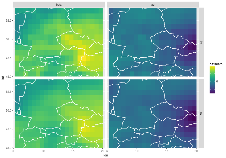
The estimation and smoothing of the regression parameters seems to work.
The estimated parameters are similar, but the fields on the bottom are smoother because we have built spatial dependency into the model.
By varying the parameter sigma2 in the function calc_x0 higher or lower degrees of smoothing can be achieved.
TODO: illustrate effect of different smoothing parameters
In-sample evaluation
The important question is now whether or not the spatial modeling has improved the transformed forecasts over independent estimation. First of all we look at the mean squared residuals of the two models, i.e. the mean squared prediction errors (MSEs) calculated on the training data:
df_mse_insample_lm = t2m_lm_mse %>% select(-mse_loo) %>% mutate(type='lm')
df_mse_insample_rw = df_out %>% group_by(s,lat,lon) %>% summarise(mse = mean(resid^2)) %>% mutate(type='rw')
df_mse_insample = bind_rows(df_mse_insample_lm, df_mse_insample_rw)

df_mse_insample %>% group_by(type) %>% summarise(mse = mean(mse)) %>% knitr::kable()
| type | mse |
|---|---|
| lm | 0.6612585 |
| rw | 0.6783852 |
It is not surprising that the in-sample residuals are smaller for the independent model than for the spatially dependent model, since sum of squared residuals is exactly the quantity that is minimised by standard linear regression. Any modification will necessarily increase the sum of squared residuals. To evaluate the models, we will have to look at their performances out-of-sample, i.e. how well they predict values of $y$ that were not part of the training data.
Out-of-sample evaluation
df_cv = t2m %>% mutate(y_hat = NA_real_)
for (yr_loo in unlist(distinct(t2m, year))) {

  # create training data set
  df_trai = t2m %>% filter(year != yr_loo)

  # estimate regression parameters
  x0 = calc_x0(sigma2=0.1, data=df_trai, lambda=1, tol=1e-4)$x0
  alpha_hat = x0[1:N_s]
  beta_hat  = x0[1:N_s + N_s]
  tau_hat   = x0[1:N_s + 2*N_s]

  # append fitted value to data frame
  df_cv = df_cv %>%
    mutate(y_hat = ifelse(year == yr_loo, alpha_hat + beta_hat * fcst, y_hat))
}
df_mse_outofsample_lm = t2m_lm_fit %>% select(s, lat, lon, year, resid_loo) %>% mutate(type='lm')
df_mse_outofsample_rw = df_cv %>% mutate(resid_loo = y_hat - obs) %>% select(s, lat, lon, year, resid_loo) %>% mutate(type='rw')
df_mse_outofsample =
  bind_rows(df_mse_outofsample_lm, df_mse_outofsample_rw) %>%
  group_by(type) %>% summarise(mse = mean(resid_loo^2))

df_mse_outofsample %>% knitr::kable()
| type | mse |
|---|---|
| lm | 0.8995776 |
| rw | 0.8524261 |
When evaluated out-of-sample in a leave-one-out cross validation, the regression model with smoothed parameters performs better than the regression model with independently fitted paramters. The improvement in mean squared error is close to $10\%$, which is substantial.
This is encouraging. Since we have not yet optimised (or integrated over) the smoothing parameter $\sigma^2$ of the 2d random walk model further improvements might be possible.
TODO:
- compare posterior standard deviations of the spatial model with standard errors of regression parameters
- explore $\sigma^2$ to estimate the posterior $p(\theta \vert y)$
- integrate over $\sigma^2$ to estimate $p(x \vert y)$
- consider different $\sigma^2$ for $\alpha$, $\beta$, and $\tau$
- consider different spatial models