INLA from scratch

Last update: 22 September 2017

INLA (integrated nested Laplace approximation) is a popular framework for approximate Bayesian inference in complicated space-time models. It can provide a significant speedup over Markov-Chain Monte-Carlo in highdimensional models.

When I started reading about INLA, I found a few technical papers in stats journals that explain the theory. When I searched for INLA on the internet to get a more gentle introduction, I got the impression that the INLA methodology is identical with the R package INLA. Every blog post or forum entry I found on INLA was dealing with issues related to the R package. I could not find any examples where someone implemented INLA (the mathematical framework) from scratch, without using the R package.

This report is my attempt to implement INLA from scratch, without using the R package. The motivation is to understand the method in more detail, and to make the R package less of a black box.

The report was written in R markdown, converted to markdown with knitr, converted to html with jekyll and hosted via github pages.

Load libraries

library(Matrix)
library(tidyverse)

## Loading tidyverse: ggplot2
## Loading tidyverse: tibble
## Loading tidyverse: tidyr
## Loading tidyverse: readr
## Loading tidyverse: purrr
## Loading tidyverse: dplyr

## Conflicts with tidy packages ----------------------------------------------

## expand(): tidyr, Matrix
## filter(): dplyr, stats
## lag():    dplyr, stats

knitr::opts_chunk$set(
  cache.path='_knitr_cache/inla-from-scratch/',
  fig.path='figure/inla-from-scratch/'
)

A toy model

Consider the case where we want to learn something about a time series that comes in the form of zeros and ones, for example

\begin{equation} (y_1, …, y_n) = (0, 1, 0, 0, 1, 1, 1, …, 0, 1) \end{equation}

Such a binary time series could occur, for example, as a record of rain/no rain on consecutive days. As is usual in meteorological time series, consecutive values are correlated with one another. For rain data, we usually observe that a rainy day is more likely to be followed by a rainy day than by a dry day. The auto-correlation structure is a useful statistical property to infer from such a time series.

How should we model a time series of auto-correlated zeros and ones? One way is to model the data by a two-stage process.

The observations $y_1, …, y_n$ are Bernoulli trials with success probabilities $p_1, …, p_n$.

\begin{equation} p(y_t | p_t) = \begin{cases} p_t & \mathrm{if}\; y_t = 1 \newline 1 - p_t & \mathrm{if}\; y_t = 0 \end{cases} \end{equation}

or equivalently

\begin{equation} p(y_t | p_t) = p_t^{y_t} (1 - p_t)^{1-y_t} \end{equation}

The unobserved success probabilities $p_1, …, p_n$ are assumed to change over time in a smooth way. We assume that $p_1, …, p_n$ depend on a latent process $x_1, …, x_n$ through a logit link:

\begin{equation} p_t = \frac{\exp(\beta x_t)}{1 + \exp(\beta x_t)} \end{equation}

This guarantees that $p_t$ is between zero and one. The latent process $x_1, …, x_n$ is a realisation of a first-order auto-regressive (AR1) process:

\begin{equation} x_t = \alpha x_{t-1} + \sigma \epsilon_t \end{equation}

where the $\epsilon_t$ are iid standard Normal variates. The conditional distribution $p(x_t|x_{t-1})$ is $N(\alpha x_{t-1}, \sigma^2)$ and the marginal distribution $p(x_t)$ is $N(0, \frac{\sigma^2}{1 - \alpha^2})$.

We refer to the hyperparameters ${\alpha, \beta, \sigma}$ collectively by $\theta$ and to their joint prior distribution as $p(\theta)$.

In the following simple example we will assume that $\beta$ and $\sigma$ are known. The goal will be to infer the posterior distribution of the AR1 parameter $\alpha$ using the INLA approximation.

Simulated data

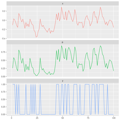
We simulate data from the toy model with parameter settings $n=100$, $\alpha=0.6$, $\sigma=0.1$, and $\beta=10$, and plot time series of $x_t$, $p_t$, and $y_t$.

set.seed(1234)
n = 100
alpha_true = .6
sigma_true = 0.1
beta_true = 10

# simulate x_t as AR1, p_t as logit(x_t), and y_t as Bernoulli(p_t)
x_true = arima.sim(n=n, model=list(ar=alpha_true), sd=sigma_true) %>% as.numeric
p_true = 1 / (1 + exp(-beta_true * x_true))
y = rbinom(n, 1, p_true)

# create data frame for plotting
df = data_frame(i = 1:n, x = x_true, p = p_true, y = y) %>% 
     gather(key='variable', value='value', -i) %>%
     mutate(variable = factor(variable, levels=c('x','p','y'))) 

# plot the time series x_t, p_t, and y_t in 3 panels
ggplot(df, aes(x=i, y=value, color=variable)) + 
  geom_line(na.rm=TRUE, show.legend=FALSE) + 
  facet_wrap(~variable, ncol=1, scales='free_y') + 
  xlim(0,100) + labs(x=NULL, y=NULL)

The joint log-likelihood

Here we derive the full joint distribution of the observations $y = (y_1, …, y_n)$, the latent process $x = (x_1, …, x_n)$ and the hyperparameters $\theta = (\alpha, \beta, \sigma)$. The full joint distribution can be factorised as follows:

\begin{equation} p(y, x, \theta) = p(y \vert x, \theta) p(x \vert \theta) p(\theta) \end{equation}

It will be convenient to work with log probabilities instead of probabilities, so the joint distribution can equivalently be expressed as

\begin{equation} \log p(y, x, \theta) = \log p(y \vert x, \theta) + \log p(x \vert \theta) + \log p(\theta) \end{equation}

The conditional log-probability of the observations is given by

\begin{align} \log p(y \vert x,\theta) & = \sum_t \left[ y_t \log(p_t) + (1 - y_t) \log(1 - p_t) \right] \newline & = \sum_t \left[ \beta x_t y_t - \log(1 + \exp(\beta x_t)) \right] \end{align}

The latent process $x$ has a multivariate Normal distribution which we derive next. $x_1$ has prior distribution $N(0,\frac{\sigma^2}{1-\alpha^2})$ and $x_2, …, x_n$ have conditional distributions according to the AR1 model. So the joint distribution of $x_1,…,x_n$ factorises as

\begin{align} p(x_1, …, x_n) & = p(x_1) p(x_2 \vert x_1) p(x_3 \vert x_2) … p(x_n \vert x_{n-1})\newline & \propto \exp \left[ -\frac{1}{2\sigma^2} \left[ x_1^2 (1 - \alpha^2) + (x_2 - \alpha x_1)^2 + (x_3 - \alpha x_2)^2 + … + (x_n - \alpha x_{n-1})^2 \right]\right]\newline & = \exp \left[ -\frac{1}{2\sigma^2} \left[ x_1^2 - 2\alpha x_1 x_2 + x_2^2 (1 + \alpha^2) - 2 \alpha x_2 x_3 + x_3^2 (1 + \alpha^2) - … + x_{n-1}^2 (1 + \alpha^2) - 2 \alpha x_{n-1} x_n + x_n^2 \right] \right]\newline & = \exp \left[ -\frac12 x’ Q x \right] \end{align}

which is a multivariate Normal distribution with zero mean and precision (inverse covariance) matrix given by

\begin{equation} Q = \frac{1}{\sigma^2} \left(\begin{matrix} 1 & -\alpha & & & \newline -\alpha & 1 + \alpha^2 & -\alpha & & \newline & \ddots & \ddots & \ddots& \newline & & -\alpha & 1 + \alpha^2 & -\alpha \newline & & & -\alpha & 1 \end{matrix}\right) \end{equation}

We don’t make any assumptions about the prior distribution $p(\theta)$ of the hyperparameters at this point. In summary, the joint log-density of the observations, latents and hyperparamaters is given by

\begin{align} \log p(y,x,\theta) = & \log p(y\vert x,\theta) + \log p(x\vert \theta) + \log p(\theta) \newline \propto &\sum_t \left[ \beta x_t y_t - \log(1 + \exp(\beta x_t)) \right] + \frac12 \log\vert Q\vert - \frac12 x’Qx + \log p(\theta) \end{align}

INLA

INLA (integrated nested Laplace approximation) is a statistical framework for Bayesian inference in models of the following form:

observations: $\log p(y \vert x,\theta) = \sum_i \log p(y_i \vert x_i, \theta)$, The distribution of the observation $y_t$ at index $t$ depends only on the value of the latent variable $x_t$. This can be relaxed, and we can say that the distribution of $y_t$ depends only on a small number of the latent variables. The distribution of the observations is assumed to be from the exponential family, but I haven’t figured out yet whether this assumption is really necessary.

latent variables: $\log p(x\vert\theta) \propto \frac12 \log\vert Q \vert - \frac12 x’Qx$. The latent variables $x_t$ are a Gauss Markov random field, which is a multivariate Normal distribution with a sparse precision matrix $Q$.

hyperparameters: $\theta \sim p(\theta)$. The prior distribution of the hyperparameters is arbitrary, but the number of hyperparameters has to be small ($< 6$).

This hierarchical model covers a wide range of statsitical models for spatial, temporal and spatio-temporal data. The reasons for the restrictions such as sparsity of $Q$ and small number of hyperparameters will become clear as we develop the framework.

Approximating the posterior $p(\theta \vert y)$

One goal of INLA is to calculate an approximation of the posterior of the hyperparameters $p(\theta | y)$. This is not trivial since the latent variables $x_1, …, x_n$ have to be integrated out. Doing this with MCMC is usually very expensive, and becomes intractable if the dimensionality $n$ is large.

We are going to proceed in two steps: We will first approximate $p(\theta | y)$ up to a multiplicative constant. Then we will use numerical integration to normalise the posterior. Since the dimensionality of $\theta$ is small, we can get away with using numerical quadrature methods such as Simpson’s rule to calculate the normalisation constant.

Observations $y$ are at fixed values, and in the following we also assume that $\theta$ is fixed at a particular value. To build up the posterior of $\theta$ we will have to apply the following for many different values of $\theta$.

From the (slightly unusual) factorisation of the joint distribution

\begin{equation} \log p(y,x,\theta) = \log p(x\vert\theta, y) + \log p(\theta\vert y) + \log p(y) \end{equation}

we get the following expression for the posterior of the hyperparameters

\begin{equation} \log p(\theta \vert y) \propto \log p(y,x,\theta) - \log p(x\vert y,\theta) \end{equation}

The symbol $\propto$ is to be read as “equal up to an additive constant” when working with log-probabilities, and “equal up to a multiplicative constant” when working with probabilities.

The above expression is valid for arbitrary values of $x$ (with non-zero density). A particularly useful choice of $x$ is to use the mode $x_0(\theta)$ of $\log p(y,x,\theta)$, i.e. the values of $x_1, …, x_n$ that maximise $p(y,x,\theta)$ at fixed values of $\theta$ and $y$. Hence we will express the posterior of the hyperparameters evaluated at the value $\theta$ as

\begin{equation} \log p(\theta \vert y) \propto \left[ \log p(y,x,\theta) - \log p(x\vert y,\theta) \right]_{x=x_0(\theta)} \end{equation}

The challenge is now to find a good approximation of the conditional distribution of the latent variables $p(x \vert y, \theta)$. In the INLA method, $p(x \vert y,\theta)$ is approximated using the Laplace approximation. The Laplace approximation approximates integrals of the form $\int dx\; e^{f(x)}$ by the following relationship:

\begin{equation} \int dx\; e^{f(x)} \approx e^{f(x_0)} (2\pi)^{n/2} \big\vert -Hf(x_0)\big\vert ^{-1/2} \end{equation}

where $x_0$ is the mode of $f(x)$, and $Hf(x_0)$ is the Hessian matrix of $f$ (i.e. the matrix $H_{ij}$ of second derivatives of $f$ with respect to $x_i$ and $x_j$) evaluated at the mode.

To apply the Laplace approximation to approximate $p(x \vert y, \theta)$, we first define the function $f(x)$ which is proportional to the log joint $\log p(y,x,\theta)$ taken as a function of $x$, i.e. at fixed values of $y$ and $\theta$. It should be emphasised that $f(x)$ is a different function for different choices of $\theta$ during the approximation of $p(\theta\vert y)$. Then the conditional $p(x \vert y,\theta)$ can be expressed through $f(x)$ by

\begin{equation} p(x\vert y,\theta) = \frac{\exp[f(x)]}{\int dx \exp[f(x)]} \end{equation}

The denominator is approximated by the Laplace approximation. So the Laplace approximation of $p(x \vert y, \theta)$ evaluated at the mode $x_0$ reads

\begin{equation} \log p(x_0 | y, \theta) \approx -\frac{n}{2} \log (2\pi) + \frac12 \log \big\vert -Hf(x_0) \big\vert \end{equation}

and the log of the posterior $p(\theta \vert y)$ is approximately proportional to

\begin{equation} \log p(\theta \vert y) \propto \log p(y, x_0, \theta) - \frac12 \log \big\vert -Hf(x_0) \big\vert \end{equation}

In our toy model, the function $f(x) \propto \log p(y,x,\theta)$ is given by

\begin{equation} f(x) = \sum_t [\beta x_t y_t - \log ( 1 + \exp(\beta x_t))] - \frac12 x’Qx \end{equation}

The gradient vector and Hessian matrix of $f$ are given by

\begin{align} \nabla f (x) & = vec\left[ \beta y_i - \frac{\beta \exp(\beta x_i)}{1+\exp(\beta x_i)}\right] - Qx\newline Hf(x) & = - Q - diag\left[ \frac{\beta^2 \exp(\beta x_i)}{(1+\exp(\beta x_i))^2} \right] \end{align}

Calculating the mode $x_0$

I haven’t talked about how the mode $x_0$ is calculated to apply the Laplace approximation. In R, one could simply use one of the out-of-the-box optimisation routines implemented in the optim function. These work in general, but are about 10 times slower than the iterative method proposed in the original paper, which I describe here:

The function $f(x)$ which we want to maximise can be written as

\begin{equation} f(x) = -\frac12 x’Qx + \sum_i g_i(x_i) \end{equation}

where $g_i(x_i) = \log p(y_i \vert x_i, \theta)$.

We Taylor expand $f(x)$ around an initial guess of the mode $x_0$, only keeping those additive terms that depend on $x$:

\begin{align} f(x) & \approx f(x_0) + \nabla f(x_0) (x-x_0) + \frac12 (x-x_0)’ Hf(x_0) (x-x_0)\newline & \propto [ \nabla f (x_0) - x_0’ Hf(x_0) ] x + \frac12 x’ Hf(x_0) x \end{align}

where $\nabla f$ and $Hf$ are gradient vector and Hessian matrix of $f(x)$. Ignoring terms that do not depend on $x$ is permissible because we only want to find the mode $x_0$ of $f(x)$ which does not change when we ignore additive and multiplicative constants.

The Taylor expansion approximates $f(x)$ by a parabola through $x_0$ that matches the first and second derivative of $f(x)$ at this point. Since $f(x)$ is proportional to $\log p(x \vert y, \theta)$, we are in fact approximating $p(x \vert y, \theta)$ by a Normal distribution. The mode of the fitted parabola is found by setting its first derivative to zero and solving for $x$, so the mode of the parabola is given by the solution to the equation

\begin{align} [Q - diag\; g^{‘‘}_i(x_0)] x = vec\; g^{‘}_i(x_0) - x_0’ diag\; g^{‘‘}_i(x_0) \end{align}

The mode of the fitted parabola provides a new, improved estimate of the true mode of $f(x)$. By repeating the process using the new improved estimate of the mode as the new test point $x_0$ of the Taylor expansion, we can find the mode of $f(x)$ iteratively.

The role of the INLA restrictions

I mentioned earlier that application of INLA is restricted to latent Gaussian models with a sparse precision matrix of the latent process, with sparse dependency between $y$ and $x$, and for small number of hyperparameters $\theta$. We can now get a better idea why these restrictions are needed.

To approximate $p(\theta \vert y)$ by INLA, we will have to evaluate $p(y, x, \theta)$, find the mode $x_0$, and Laplace approximation of $p(x\vert y,\theta)$, each at many different values of $\theta$. The most expensive steps involve the matrix $Q$, i.e. to calculate the determinant of $Q$, the quadratic form $x’Qx$, and the determinant of the Hessian, which also involves $Q$. If the matrix $Q$ is sparse, the complexity of calculating the determinant and quadratic form reduces dramatically compared to a dense matrix. This is why we use Gauss-Markov random fields to model the latent process $x$.

The Hessian of $f(x)$ is the sum of the sparse matrix $Q$ and the matrix of second derivatives of the conditional log density of the observations given $x$. If each $y_t$ only depends on a small number of latent variables $x_t$ the matrix of second derivatives will be sparse, and therefore the Hessian is sparse as well which makes calculation of the determinant in the Laplace approximation efficient.

Lastly, by limiting the number of hyperparameters $\theta$, the number of evaluations of the INLA algorithm is limited to a manageable amount, and numerical integration by simple quadrature isn’t too expensive.

R functions

So let’s implement INLA for our toy model. We will assume that the parameters $\beta=10$ and $\sigma = 0.1$ are known, and the unknown parameter to be inferred is the AR1 parameter $\alpha$ of the latent process.

We next define the necessary R functions.

The sparse precision matrix $Q$

calc_Q = function(alpha) {
  1 / sigma_true^2 * Matrix::bandSparse(n, k=0:1, 
    diagonals = list(c(1, 1 + alpha^2, 1) %>% rep(c(1, n-2, 1)), 
                     -alpha %>% rep(n-1)), 
    symmetric=TRUE)
}

The log prior for $\alpha$

The AR1 coefficient is between -1 and 1. We assume a beta prior for $(\alpha + 1) / 2$, with default values set to 1 so the prior is uniform.

calc_lprior = function(alpha, a=1, b=1) {
  (a-1) * log((alpha + 1) / 2) + (b-1) * log(1 - (alpha+1)/2)
}

The log joint distribution $p(y,x,\theta)$

We calculate the determinant of $Q$ from its Cholesky decomposition $Q = L’L$ ($L$ is an upper triangular matrix). We use the identity $\vert Q\vert = \prod L_{ii}^2$ and equivalently $\log \vert Q\vert = 2 \sum_i \log L_{ii}$:

calc_ljoint = function(y, x, alpha, a=1, b=1) {
  chol_Q = calc_Q(alpha) %>% chol
  logdet_Q_half = chol_Q %>% diag %>% log %>% sum
  quad_form = crossprod(chol_Q %*% x) %>% drop
  res = 
    sum(beta_true * x * y - log1p(exp(beta_true * x))) + 
    logdet_Q_half - 0.5 * quad_form + 
    calc_lprior(alpha, a, b)
  return(res)
}

The function $f(x)$, its gradient and its negative Hessian

calc_ff = function(x, alpha) {
  sum(beta_true * x * y - log1p(exp(beta_true * x))) - 
  0.5 * drop(as.matrix(x %*% calc_Q(alpha) %*% x))
}

calc_grad_ff = function(x, alpha) {
  beta_true * y - 
  beta_true * exp(beta_true * x) / (1 + exp(beta_true * x)) - 
  drop(as.matrix(calc_Q(alpha) %*% x))
}

calc_neg_hess_ff = function(x, alpha) {
  calc_Q(alpha) + 
  diag(beta_true^2 * exp(beta_true * x) / (1 + exp(beta_true * x))^2)
}

Calculate the mode of $f(x)$

# the function g(x) = log(p(y | x,theta)), its gradient and hessian
calc_g0 = function(x) {
  sum(beta_true * x * y - log1p(exp(beta_true * x)))
}
calc_g1 = function(x) {
  beta_true * y - beta_true * exp(beta_true * x) / (1 + exp(beta_true * x)) 
}
calc_g2 = function(x) {
  (-1) * beta_true^2 * exp(beta_true * x) / (1 + exp(beta_true * x))^2
}

calc_x0 = function(alpha, tol=1e-12) {
  Q = calc_Q(alpha)
  x = x0 = rep(0, n)
  while(1) {
    g1 = calc_g1(x)
    g2 = calc_g2(x)
    x = drop(solve(Q - bandSparse(n=n, k=0, diagonals=list(g2))) %*% 
             (g1 - x0 * g2))
    if (mean((x-x0)^2 < tol)) {
      break
    } else {
      x0 = x
    }
  }
  return(x)
}

Here is a brute force optimisation using the built-in R function optim, which is 10 times slower than the iterative method above, but gives the same result:

calc_x0_brute = function(alpha) {
  optim(par=rep(0, n), fn=calc_ff, gr=calc_grad_ff, alpha=alpha, 
        control=list(fnscale=-1), method='BFGS')$par
}

Approximating the log posterior up to an additive constant

With the above functions, approximating $\log p(\theta\vert y)$ up to an additive constant is straightforward:

calc_lpost = function(alpha) {
  x0 = calc_x0(alpha)
  chol_h = chol(calc_neg_hess_ff(x0, alpha))
  calc_ljoint(y, x0, alpha) - sum(log(diag(chol_h)))
}
alpha_vec = seq(-.95, .95, len=31)
lpost = sapply(alpha_vec, calc_lpost) 

Normalisation of the posterior

Once $p(\theta\vert y)$ is approximated up to a constant, we can use numerical integration such as Simpson’s rule to find the normalisation constant. Here is an implementation using the composite Simpson’s rule:

calc_Z = function(alpha_vec, lpost_vec) {
  nn = length(alpha_vec)
  hh = alpha_vec[2] - alpha_vec[1]
  ww = c(1, rep(c(4,2), (nn-3)/2), c(4,1))
  return(sum(ww * exp(lpost_vec)) * hh / 3)
}

Putting it all together

At this point, approximation of the unnormalised log posterior of $\alpha$ is a simple matter of an sapply call, and the normalisation constant can be approximated subsequently:

lpost = lpost - mean(lpost) # to avoid numerical overflow
Z = calc_Z(alpha_vec, lpost)

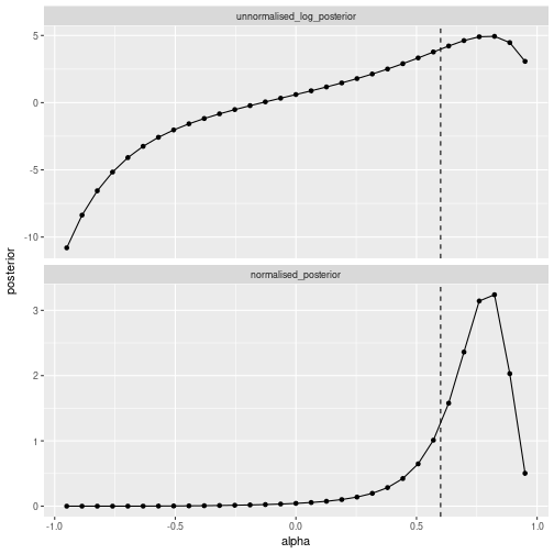
We plot the unnormalised log-posterior and the normalised posterior:

# data frame for plotting
df_posterior = 
  bind_rows(
    data_frame(alpha=alpha_vec, posterior=lpost, 
               type='unnormalised_log_posterior'),
    data_frame(alpha=alpha_vec, posterior=exp(lpost)/Z, 
               type='normalised_posterior')) %>% 
  mutate(type = factor(type, levels=c('unnormalised_log_posterior', 
                                      'normalised_posterior')))

# plot unnormalised log posterior and normalised posterior in 2 panels
ggplot(df_posterior, aes(x=alpha, y=posterior)) + 
  geom_line() + geom_point() +
  geom_vline(aes(xintercept=alpha_true), linetype='dashed') + 
  facet_wrap(~type, scale='free_y', ncol=1) +
  theme(legend.position='none')

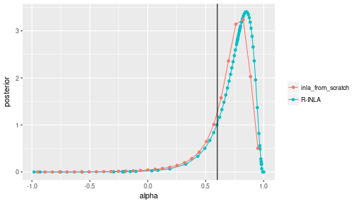
Comparison with R-INLA

For comparison we use the R package INLA to calculate the posterior $p(\alpha\vert y)$.

The AR1 parametrisation in R-INLA

In R-INLA, the AR1 latent model is parametrised through the parameters $\theta_1$ and $\theta_2$. $\theta_1$ is the log marginal precision of the AR1 process, i.e. using our notation $\theta_1 = \log[ (1 - \alpha^2) / \sigma^2]$. Since we only want to infer the AR1 parameter $\alpha$, we fix $\theta_1$ at its true value in the R-INLA prior specification. The parameter $\theta_2$ is the logit transformed AR1 parameter, i.e. using our notation $\theta_2 = \log[ (1+\alpha) / (1-\alpha) ]$. R-INLA specifies a Normal prior for $\theta_2$, whereas we have specified a uniform (Beta(1,1)) prior for $\alpha$.

The R-INLA default prior for $\alpha$

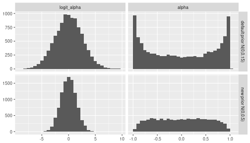
It is worthwhile to have a look at the default $N(0,1/0.15)$ prior for $logit(\alpha)$ used by R-INLA (the documentation of the AR1 model in R-INLA can be found here). Judging from the figure below, this is a rather curious choice for a default prior, as it will strongly bias the posterior of $\alpha$ away from zero, towards +1 and -1. Based on exploratory analysis, we will choose a different prior for $\theta_1$, namely $N(0, (1/0.5))$ which yields a distribution over $\alpha$ that is much closer to uniform. Note that a completely uniform distribution for $\alpha$ cannot be achieved with a Normal prior on $logit(\alpha)$.

# data frame for plotting
df_prior = 
  bind_rows(
    data_frame(logit_alpha = rnorm(1e4,0,sqrt(1/0.15)), 
               type='default prior N(0,0.15)'), 
    data_frame(logit_alpha = rnorm(1e4,0,sqrt(1/0.5)), 
               type='new prior N(0,0.5)')) %>% 
  group_by(type) %>% 
  mutate(alpha = (exp(logit_alpha)-1)/(exp(logit_alpha) + 1)) %>%
  ungroup %>%
  gather(key='transformation', value='value', -type) %>%
  mutate(transformation = factor(transformation, levels=c('logit_alpha', 'alpha'))) 

# plot distributions of logit(alpha) and alpha for the two priors in 4 panels
ggplot(df_prior, aes(x=value)) + 
  geom_histogram(bins=30) + 
  facet_grid(type ~ transformation, scale='free') +
  labs(x=NULL, y=NULL)

The R-INLA implementation

library(INLA)

## Loading required package: sp

## Loading required package: methods

## This is INLA_17.06.20 built 2017-09-07 09:01:27 UTC.
## See www.r-inla.org/contact-us for how to get help.

theta1_true = log((1-alpha_true^2)/sigma_true^2) 
theta2_param = c(0, 0.5)
A_mat = diag(beta_true, n, n) %>% inla.as.sparse

inla_formula = 
  y ~ -1 + 
      f(i, model='ar1', hyper=list(
        theta1 = list(fixed=TRUE, initial=theta1_true),
        theta2 = list(param=theta2_param)))
inla_data = data_frame(i=1:n, y=y)

res = inla(
  formula=inla_formula, 
  data=inla_data, 
  family='binomial', 
  Ntrials=rep(1,n), 
  control.predictor=list(A = A_mat)
)

## Note: method with signature 'Matrix#numLike' chosen for function '%*%',
##  target signature 'dgTMatrix#numeric'.
##  "TsparseMatrix#ANY" would also be valid

## Note: method with signature 'sparseMatrix#matrix' chosen for function '%*%',
##  target signature 'dgTMatrix#matrix'.
##  "TsparseMatrix#ANY" would also be valid

# data frame for plotting
df_compare = bind_rows(
  res$marginals.hyperpar$`Rho for i` %>% 
    as_data_frame %>%
    rename(alpha=x, posterior=y) %>%
    mutate(type='R-INLA'),
  data_frame(alpha=alpha_vec, posterior=exp(lpost) / Z) %>% 
    mutate(type='inla_from_scratch')
)

# plot posteriors for inla-from-scratch and R-INLA 
ggplot(data=df_compare, mapping=aes(x=alpha, y=posterior, colour=type)) + 
  geom_line() + geom_point() +
  geom_vline(aes(xintercept=alpha_true)) + 
  labs(color=NULL)

Approximating the posterior of the latent variables $p(x \vert y)$

The posterior of the latent variables can be calculated by

\begin{equation} p(x \vert y) = \int d\theta\; p(x \vert y, \theta) p(\theta \vert y) \end{equation}

which can be approximated numerically by a finite sum

\begin{equation} p(x \vert y) \approx \sum_i p(x \vert y, \theta_i) p(\theta_i \vert y) \Delta_i \end{equation}

While building up the approximation of $p(\theta \vert y)$ we have approximated the conditional distribution $p(x \vert y, \theta)$ by a Normal distribution at many different values of $\theta$. Assume we save all those Normal approximations (i.e. the means and precision matrices) during the approximation of $p(\theta \vert y)$. Then we approximate $p(x \vert y)$ by a mixture of Normal distributions with weights given by $p(\theta_i \vert y) \Delta_i$.

We will probably be interested in marginal variances of the individual $x_t$. To get those we have to invert the precision matrices of the Normal distributions in the mixture to get the covariance matrix. Then we can calculate each marginal posterior mean and variance as mean and variance of a Normal mixture through the relations

\begin{align} E[X] & = \mu = \sum_i w_i \mu_i \newline E[(X-\mu)^2] & = \sigma^2 = \sum_i w_i ((\mu_i - \mu)^2 + \sigma_i^2) \end{align}

where $w_i$ are the weights, $\mu_i$ are the individual means of the mixture components, and $\sigma_i^2$ are their individual variances.

Below we go through the whole process of approximating $p(\theta \vert y)$ once again to get a self-contained function to approximate the marginals $p(x_t \vert y)$. In a proper implementation, $p(\theta \vert y)$ and $p(x \vert y)$ can obviously be inferred in one pass.

# approximate p(x | y, alpha) for many values of alpha
alpha_vec = seq(-.95, .95, len=31)
post_x = lapply(alpha_vec, function(alpha_) {
  mode_ = calc_x0(alpha_)
  chol_H_ = chol(calc_neg_hess_ff(mode_, alpha_))
  # save alpha, the mode, the covariance matrix, and p(theta|y) unnormalised
  return(list(
    alpha = alpha_, 
    x0 = mode_,
    diag_sigma = drop(diag(chol2inv(chol_H_))),
    unn_log_post = calc_ljoint(y, mode_, alpha_) - sum(log(diag(chol_H_)))
  ))
})

# extract marginal means and variances for each p(x|y,theta)
mu = sapply(post_x, `[[`, 'x0')
sigma2 = sapply(post_x, `[[`, 'diag_sigma')

# normalise the posterior
lpost = sapply(post_x, `[[`, 'unn_log_post')
lpost = lpost - mean(lpost) # to avoid numerical overflow
post_alpha = exp(lpost) / calc_Z(alpha_vec, lpost)

mu_post = sapply(1:n, function(ii) weighted.mean(mu[ii,], w=post_alpha))
sigma_post = 
  sapply(1:n, function(ii) 
    weighted.mean((mu[ii,] - mu_post[ii])^2 + sigma2[ii,], w=post_alpha)
  ) %>% 
  sqrt

# data frame for plotting
df_latent = bind_rows(
  data_frame(
    type = 'inla_from_scratch', i=1:n, mu = mu_post, 
    lwr = mu_post - 2 * sigma_post, 
    upr = mu_post + 2 * sigma_post),
  data_frame(
    type = 'R-INLA', i=1:n, mu = res$summary.random$i[,'mean'],
    lwr = with(res$summary.random$i, mean - 2 * sd),
    upr = with(res$summary.random$i, mean + 2 * sd)),  
  data_frame(
    type = 'truth', i=1:n, mu = x_true, lwr = x_true, upr = x_true)
) 

# ribbon plots for p(x|y) for inla-from-scratch and R-INLA, and true values
ggplot(df_latent, aes(x=i)) + 
  geom_ribbon(aes(ymin=lwr, ymax=upr, alpha=type, linetype=type, color=type), 
              fill=NA) +
  geom_line(aes(y=mu, color=type)) + labs(alpha=NULL, linetype=NULL, color=NULL, x=NULL, y=NULL)

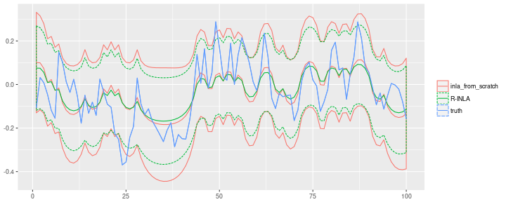
Differences to R-INLA

My results are close, but not identical to the results obtained with the R package. The best explanation for the difference is, of course, that I made a mistake somewhere along the way. But even if my implementation is correct, we should expect differences.

The prior I used was similar, but not identical to prior in R-INLA. I tried slightly larger sample sizes to suppress the influence of the prior, but the two solutions do not seem to converge. Due to the hierarchical structure of the model, there seems to be some irreducible uncertainty about $\alpha$ when trying to infer it from $y$. So the posterior never becomes infinitely sharp even with huge sample sizes. I found that both my posterior and the R-INLA posterior cover the true $\alpha$ equally well, but at the same time the two distributions don’t perfectly cover each other.

R-INLA is much cleverer than I am when selecting the points at which to evaluate $p(\theta \vert y)$. I just used equally spaced points that cover the entire domain $(-1, 1)$. R-INLA samples more points close to the mode, and less points in the boring region below zero where the posterior density is vanishingly low.

The posterior of the latent process $x_t$ differs as well. This can partly be explained by the slightly different priors. But (as far as I know) R-INLA also implements a third-order correction to improve upon the Laplace approximation of $p(x \vert y, \theta)$. Furthermore, I evaluated the posterior $p(\theta \vert y)$ at different $\theta$ values than R-INLA. Since the $p(\theta_i \vert y)$ enter as weights in the Normal mixture distribution some differences are to be expected as well. My posterior means are less smooth than the R-INLA means, which is consistent with my posterior mean for $\alpha$ being smaller than that of R-INLA. Also, my credible intervals are wider than those of R-INLA.

Lastly, the capabilities of R-INLA are not limited to what I showed here. R-INLA can compute posterior predictive distributions for future values of $y_t$, posterior distibutions of transformed variables, and much more.

Conclusions

INLA is an efficient method for approximate Bayesian inference in latent Gaussian models with sparse dependency structure. The crucial step is to approximate the conditional distribution of the latent process $p(x \vert y, \theta)$ by a Normal distribution. This approximation reduces the computational complexity in high-dimensional problems, and leads to semi-analytic solutions of posterior distributions that are of interest in Bayesian inference. The framework is applicable to a wide range of hierarchical Bayesian models, with a few sparsity constraints on the dependency structure.

The INLA framework is not identical to the R package INLA, that is, you do not have to install the R package to apply INLA. I showed how to implement INLA to approximate the posterior distribution of the autocorrelation parameter of a simple AR1-Bernoulli process. The results broadly agree with the results obtained with the R package.