out %>% as.data.frame %>% pivot_longer(c(dose, gi, blood), names_to='compartment', values_to='amount [g]') %>% filter(time <= 5) %>% ggplot() + geom_line(aes(x=time, y=`amount [g]`, colour=compartment))

In this note I will discuss and code a pharmacokinetic compartment model of how alcohol (or some other substance) moves through the human body. This model is part of a series of simulation models that I'm using in a course on Uncertainty Quantification.
Pharmacokinetics studies how chemical substances such as toxins or drugs move through the body over time, starting with initial exposure or administration, to their distribution to different parts of the body, to eventual elimination through metabolism or excretion. Compartment models are a class of pharmacokinetic models in which the body is conceptualised as a small number of discrete, interconnected compartments, and the substance moves between compartments and is eliminated from them at different rates.
For example, alcohol is (usually) orally administred, and so initially enters the body through the gastro-intestinal (GI) tract. From there it is absorbed into the blood-brain system where it produces its effects. From the blood, alcohol is also moved to the liver where it is eliminated through metabolic processes. The pharmacokinetics of alcohol can thus be modelled using two compartments: The GI tract and the blood/brain system. The concentration of alcohol over time in each compartment is determined by the amount ingested, and by how quickly that amount is exchanged between compartments and eliminated from them.
The flow between compartments in compartment models is usually described mathematically through coupled differential equations. Let \(S_G\) be the amount of alcohol in the gastro-intestinal tract, and \(S_B\) the amount in the blood. Then we can model their change over time by the system of ordinary differential equation: $$\frac{dS_G}{dt} = -k_a S_G(t) - k_g S_G(t) + D(t)$$ and $$\frac{dS_B}{dt} = k_a S_G(t) - k_e S_B(t).$$
The equation for \(S_G\) says that the rate of change of alcohol in the GI tract is proportional to the current amount \(S_G\) in the GI tract, and the rate \(D(t)\) at which alcohol currently enters the system from outside. The dependence on \(S_G(t)\) is split up into two parts: Absorption into the blood (with rate parameter \(k_a\)) and elimination from the GI tract through other processes (with rate parameter \(k_g\)). The higher the current amount \(S_G\), the faster its decrease.
The second differential equation for \(S_B\) says that the rate of change of alcohol in the blood is proportional to how much is currently in the GI tract (\(S_B\)) and how much is currently in the blood (\(S_B\)). The increase of alcohol in the blood is equal to the inflow from the GI tract (\(k_a S_G(t)\)). The term \(-k_e S_B(t)\) describes elimination of alcohol from the blood, e.g. by the liver. The higher the current amount, the faster the rate of elimination.
Let's simulate this model. The full R code for the simulation can be downloaded here: alc.R. Below I will go over the code step by step and finish with a quick comment on how "realistic" the model is.
We will use the R library "deSolve" to numerically solve the system of differential equations given the initial state and model parameters. Tidyverse is used for data wrangling and plotting.
library(tidyverse)
library(deSolve)
To simulate the model we have to specify an initial state \(S_G(0)\) and \(S_B(0)\), as well as the dosing function \(D(t)\), and the rate parameters \(k_a\), \(k_g\) and \(k_e\). For the dosing function, we will assume that alcohol flows into the system at a constant rate for a fixed amount of time, and stops afterwards. So the dosing function is specified by a duration (in hours) and a rate of flow (in grams per hour). The rate parameters are more difficult to set and usually have to be estimated by fitting the model to data. Here I use values that I determined by a quick trial and error.
# model parameters
parameters = c(
  k_g = 1.0,      # per hour, GI tract elimination rate (not into blood)
  k_a = 2.0,      # per hour, absorption rate from GI tract into blood
  k_e = 3.0,      # per hour, elimination rate from blood by liver
  duration = 0.5, # hours of dosing
  input = 28      # grams of alcohol per hour of dosing
)
For the initial state at time \(t=0\) we assume the total amount of alcohol consumed, the amount in the GI tract and the amount in the blood are all zero.
# initial state
state = c(dose = 0, gi = 0, blood = 0)
Next we have to define a function that takes as inputs the current state and model parameters, and returns the derivatives according to the right hand sides of the model differential equations. The odeSolve library requires that function to be in the following form:
# this is the 2-compartment differential equations model function, implemented
# in the correct format to be used with deSolve
model = function(t, state, parameters) {
  # state: (dose, gi, blood)
  # parameters: (k_g, k_a, k_e, duration, input)
  with(as.list(c(state, parameters)),{
    dose = ifelse(t <= duration, input, 0)  # dosing
    dgi = -k_a * gi - k_g * gi + dose   # GI tract equation
    dblood = k_a * gi - k_e * blood     # blood equation
    return(list(c(dose, dgi, dblood)))  # derivatives
  })
}
With that function defined we can use one of the many solvers implemented in odeSolve to approximate a solution to the system of differential equations over a specified amount of time. Here we use the "ode()" function, which is invoked as follows.
# simulate model for 12 hours
times = seq(0, 12, by = 0.05)
out = ode(y = state, times = times, func = model, parms = parameters)
head(out)
##      time dose       gi      blood
## [1,] 0.00  0.0 0.000000 0.00000000
## [2,] 0.05  1.4 1.300058 0.06337978
## [3,] 0.10  2.8 2.419029 0.22982663
## [4,] 0.15  4.2 3.382137 0.46939818
## [5,] 0.20  5.6 4.211091 0.75849853
## [6,] 0.25  7.0 4.924578 1.07867640
For plotting with ggplot we transform the matrix into a long data frame and then plot time series of amount ingested, amount in GI tract and amount in blood:
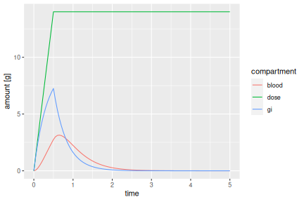
out %>%
  as.data.frame %>%
  pivot_longer(c(dose, gi, blood),
               names_to='compartment',
               values_to='amount [g]') %>%
  filter(time <= 5) %>%
  ggplot() +
    geom_line(aes(x=time, y=`amount [g]`, colour=compartment))
The total amount consumed (dose) increases linearly by 28 grams per hour for half an hour, that is, to 14 grams total, and then remains constant. The GI tract amount initially increases in the same way as the dosing function. But the full 14 grams ingested are never reached in the GI tract because of the elimination (with rate \(k_g\)), and the absorption into the blood (with rate \(k_a\)). The blood alcohol amount increases slowly because of the finite transfer rate from GI tract into blood. When the dosing stops after half an hour, the GI tract concentration starts to decrease. But blood concentration still increases for a while, before it also starts dropping due to elimination in the liver (with rate \(k_e\)).
The amount of alcohol in the blood is what will ultimately matter for the physiological effect of the ingested alcohol. Even though a total of 14 grams have been ingested in this simulation, the largest amount ever present in the blood is only about 3 grams. What effect can we expect from that amount? This will depend on the size of the person.
According to wikipedia the short term effects of alcohol consumption depent on Blood Alcohol Content (BAC), where a BAC below 0.03 produces no noticable effects, a BAC between 0.03 and 0.06 produces mild euphoria and relaxation, BAC from 0.06 to 0.1 produces disinhibition, extraversion, impaired reasoning, BAC between 0.1 and 0.2 results in boisterousness, spins, slurred speech, vomiting. By definition, a BAC of 1.0 means there is 1 gram of alcohol for each 100ml of blood, or 10g/l.
Men have about 0.075 litres of blood per kg body weight, and women have about 0.065l/kg. So, for example, an average 80kg male has about 6 litres of blood. Having 3 grams of alcohol in his blood thus puts him at \(0.5g/l\), or a BAC of 0.05. This is in the mild euphoria/relaxation range of BAC.
The total amount of alcohol consumed in this simulation is 14 grams, which corresponds to approximately one pint of beer. So the simulation with these model parameters says that an 80kg male can expect to feel slightly "tipsy" after drinking one beer, and the effect wears off after about 1.5 hours. I think this is pretty realistic.
But how were those parameter values determined? And could other parameter settings also produce "realistic" model simulations? These are questions from the field of model calibration, which I will discuss at another time.