Stefan Siegert

ggplot calligraphy

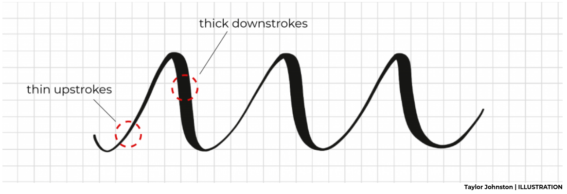
One of the characteristic effects used in hand lettering and calligraphy is to vary the line width by being light on upstrokes and using more pressure on downstrokes.

Here I'm using the R package ggplot2 (and a bit of data wrangling with dplyr), to create that effect in data visualisation:

library(ggplot2)
library(dplyr)

The ggplot command allows to map variables to different geometric properties, such as x and y coordinates, but also things like colour, and, yes, line thickness.

We first have to create a data frame with the x and y coordinates defining points along our curve. We also add a third variable that is used to modulate line width along the curve. To encode "thin on the upstroke" we set this variable constant whenever the y-coordinate increases. For a smooth transition from a light upstroke to a heavy downstroke, we make linewidth proportional to the y-change whenever the y-value decreases.

A simple curve

My first test function is the function \[y = f(x) = \sin(2x)\ e^{-0.1 x^2}\] I define a data frame that contains x and y values along the function as columns, and add a third column called lwd defined by the differenced y values truncated from above at zero.

df = tibble(x = seq(-3*pi, 3*pi, .01),
            y = sin(2*x) * exp(-.1 * x^2),
            lwd = c(NA, -pmin(diff(y), 0))) %>%
     na.omit

The lwd column is zero whenever diff(y), the change of the y variable, is positive, when the line goes up. And lwd is equal to the y-change when it is negative, i.e. on the downstroke. I multiply by minus one because I want the line to be thicker the more negative the y-change is. I also remove legend and axes to show only the line.

ggplot(df) +
  geom_path(aes(x=x, y=y, size=lwd), show.legend=FALSE) +
  theme_void()

Very nice!

A parametric 2d-curve

The function \(f(x)\) can't loop around in the x-direction. To get that, we have to use a parametric curve, for example \[\begin{aligned} x(t) & = \cos(t) - 0.1\ t\\ y(t) & = \sin(t) \end{aligned}\] where the parameter \(t\) increases over some suitable range.

df = tibble(t = seq(-4.5*pi, 3.7*pi, .01),
            x = .3 * cos(t) + .1 * t,
            y = sin(t),
            lwd = c(NA, -pmin(diff(y),-0.003))) %>%
     na.omit
ggplot(df) +
  geom_path(aes(x=x, y=y, size=lwd),
            show.legend=FALSE, lineend='round') +
  theme_void()

llllovely!

I've set the threshold when the linewidth goes constant to a small negative value rather than 0, so that the line gets to minimum thickness shortly before the minimum or maximum is reached.

I've also specified linened='round' in geom_path to avoid little cracks between between line segments and make transition between them smoother.

More parametric curves

Here is a calligraphic Lissajous curve:

df = tibble(t = seq(-2*pi, 2*pi, .01),
            x = cos(3 * t),
            y = sin(2 * t),
            lwd = c(NA, -pmin(diff(y), -0.005))) %>%
     na.omit
ggplot(df) +
  geom_path(aes(x=x, y=y, size=lwd), show.legend=FALSE, lineend='round') +
  theme_void()

... and a calligraphic hypotrochoid

RR = 7
rr = 3
dd = 6
df = tibble(t = seq(0, 10*pi, .01),
            x = (RR - rr) * cos(t) + dd * cos((RR-rr)/rr * t),
            y = (RR - rr) * sin(t) - dd * sin((RR-rr)/rr * t),
            lwd = c(NA, -pmin(diff(y),-0.01))) %>%
     na.omit
ggplot(df) +
  geom_path(aes(x=x, y=y, size=lwd), show.legend=FALSE) +
  theme_void() +
  scale_size_continuous(range=c(.4,2.5))

On that last one I used scale_size_continuous to change the minimum and maximum line width.

Random curves

There are many ways to create random 2d curves. Here I start by simulating two random walks (one for the x coordinate and one for the y coordinate) with cumsum(rnorm(n)). Then I smooth the random walks with smooth.spline. Not all random curves look good, and I had to play with the random seed and degrees of freedom parameters a bit to get a curve that I liked.

n = 1000
set.seed(187)
df = tibble(
  x = smooth.spline(cumsum(rnorm(n)), df=15)[[2]],
  y = smooth.spline(cumsum(rnorm(n)), df=15)[[2]],
  lwd = c(NA, -pmin(diff(y),0))) %>%
     na.omit
ggplot(df) +
  geom_path(aes(x=x, y=y, size=lwd),
            show.legend=FALSE, lineend='round') +
  theme_void() +
  scale_size_continuous(range=c(.5,3))