Ten years ago the "Helmhurts" blog post was published, claiming you can use the laws of electrodynamics and numerical simulation to optimally position your Wifi router. This note is an attempt to reproduce this work, deriving the necessary equations from first principles, and including all the necessary code. To make things even worse, this is completely written in R.
Here are Maxwell's equations:
The legend has it that this is what God said on the first day, and then there was light. The important quantities here are the electric field \(E\) and magnetic field \(B\), both are in general vectors that vary with space and time. The Greek letters are parameters some of which vary across space, and I'll have more to say about them later.
Our goal is to derive a relatively simple differential equation that describes the spatial variation of the electric field, considering that there is a source somewhere in space (the wifi router), the emitted wave wants to propagate through space, but there are walls that absorb and reflect it.
We start by taking the curl of Faraday's Law of Induction and substituting Ampere's Law \[\begin{aligned} \nabla \times (\nabla \times E) & = -\partial_t (\nabla \times B)\\ & = -\mu_0 \sigma \partial_t E - \mu_0 \epsilon_0\epsilon_r \partial^2_t E \end{aligned}\]
According to the "curl of the curl" law, we have \(\nabla \times (\nabla \times E) = \nabla(\nabla \cdot E) - \nabla^2 E\), so after some reshuffling of terms we get \[\nabla^2 E -\mu_0\sigma \partial_t E - \mu_0 \epsilon_0 \epsilon_r \partial^2_t E = \nabla(\nabla \cdot E)\]
which has the form of a damped inhomogenous wave equation. A common way to solve this type of equation is to assume that \(E\) is separable, that is, can be written as the product of a function only of spatial coordinates \(x\) and a function only of time: \[E(x,t) = E(x)E(t).\] Further, we assume that the time-part \(E(t)\) just oscillates harmonically with some angular frequency \(\omega\), that is, \(E(t) = e^{i\omega t}\). Substituting that separable solution into the wave equation, we get \[\nabla^2 E(x) + (\omega^2 \mu_0 \epsilon_0 \epsilon_r - i\omega \mu_0 \sigma) E(x) = \nabla(\nabla \cdot E(x))\] By reparametrising and redefining some terms (and skipping quite a few tedious details) the equation can be written as \[\nabla^2 E(x) + \left(\frac{k^2}{n(x)^2} - ik d(x)\right) E(x) = f(x),\]
where
You will have noticed the imaginary unit \(i\) in front of the damping term, which means that the solution for \(E(x)\) will be complex. To simplify the mathematical treatment we separate \(E(x)\) into real and imaginary part \(E(x) = E^{(re)}(x) + i E^{(im)}(x)\), and assume that \(n(x)\), \(d(x)\) and \(f(x)\) are all real-valued. In that way we get two coupled differential equations for real and imaginary part of \(E(x)\): \[\nabla^2 E^{(re)}(x) + \frac{k^2}{n(x)^2} E^{(re)}(x) - k d(x) E^{(im)}(x) = f(x)\] and \[\nabla^2 E^{(im)}(x) + \frac{k^2}{n(x)^2} E^{(im)}(x) + k d(x) E^{(re)}(x) = 0.\]
To solve these equations numerically, I first cut 2d space into a regular grid with grid spacing \(Delta\), so \(E^{(re)}(x)\) becomes \(E^{(re)}_{i,j}\) for row index \(i\) and column index \(j\), and the same for \(E^{(im)}\). In that discretised form the differential equation for \(E^{(re)}\) becomes \[ \frac{1}{\Delta^2} \left[E^{(re)}_{i-1,j} + E^{(re)}_{i+1,j} + E^{(re)}_{i,j-1} + E^{(re)}_{i,j+1} - 4 E^{(re)}_{i,j}\right] + \frac{k^2}{n_{i,j}^2} E^{(re)}_{i,j} - k d_{i,j} E^{(im)}_{i,j} = f_{i,j}\] and similarly for \(E^{(im)}\).
In the code below I discretise space into a regular grid with \(m\) rows and \(n\) columns. I then vectorise the 2d fields \(E^{(re)}\) and \(E^{(im)}\) by column stacking, stack these vectors on top of each other into a single vector \(E\) of length \(2mn\). Then the discretised wave equations for real and imaginary part can be written as a single linear equation \[ DE = F \] where \(D\) is a sparse matrix and \(F\) is a vector that contains the source term. We can then solve this equation for \(E\) using a sparse solver. The solution of \(E\) is devectorised into two 2d fields. I calculate the total field strength as \(\sqrt{(E^{(re)}_{i,j})^2 + (E^{(im)}_{i,j})^2}\) in each grid cell and visualise the result.
library(tidyverse)
library(Matrix)
#
# rectangular domain
m = 200
n = 200
delta = 0.02 # grid constant in metres
#
# define source term (5x5 region, arbitrary units)
f = rep(0, 2*m*n)
for (wi in 1:5) {
  for (wj in 1:5) {
    f[floor((80+wj-1)*m+20+wi)] = 1
  }
}
#
# define outer walls and inner wall with door
i_wall = c()
for (w in 1:10) {
  i_wall = c(i_wall,
    floor((w - 1)*m + 1:m),
    floor((n - w)*m + 1:m),
    floor((1:n - 1)*m + w),
    floor((1:n - 1)*m + m-w+1),
    floor((n/2 + w - 1)*m + c(1:(0.6*m),(0.8*m):m)))
}
#
# refractive index (real-valued)
# n = 1 in air larger in wall
nn = rep(1, m*n)
nn[i_wall] = 1.5
#
# damping factor (real-valued)
# d = 0 in air, larger in wall
dd = rep(0, m*n)
dd[i_wall] = 3
#
# angular frequency omega and wave number k = omega / c
freq = 2.4e9
omega = 2*pi*freq
k = omega / 3e8
#
# differential operator, discretised by finite differencing
# d2x E_re + (k/n)^2 E_re - k * d * E_im = f
# d2x E_im + (k/n)^2 E_im + k * d * E_re = 0
#
# construct off-diagonal elements of discretised laplacian:
# summation of nearest neighbors, divided by delta^2.
# for sparse matrix calculate triplets (from, to, value)
offdiags =
  tibble(
    # 2d grid points
    i = rep(1:m, n),
    j = rep(1:n, each=m),
    # 2d neighbors
    im1 = ifelse(i==1, NA, i-1),
    ip1 = ifelse(i==m, NA, i+1),
    jm1 = ifelse(j==1, NA, j-1),
    jp1 = ifelse(j==n, NA, j+1),
    # vectorised grid points
    ij = (j-1)*m + i,
    # vectorised neighbors (NA if outside domain)
    imj = (j-1)*m + im1,
    ipj = (j-1)*m + ip1,
    ijm = (jm1-1)*m + i,
    ijp = (jp1-1)*m + i) |>
  select(ij, imj, ipj, ijm, ijp) |>
  pivot_longer(-ij, names_to='delete_me', values_to='to') |>
  drop_na() |>
  select(-delete_me) |>
  rename(from=ij) |>
  mutate(value = 1/delta^2)
#
# diagonals: -4/delta^2 from discrete laplacian
# plus (k/n)^2 from linear term
diags = tibble(
  i = rep(1:m, n),
  j = rep(1:n, each=m),
  from = (j-1)*m + i,
  to = from,
  value = - 4/delta^2 + k^2 / nn^2)
#
# construct sparse matrix for the pure wave equation
# this operator is applied both to real and imag. part of E
all_entries = bind_rows(diags, offdiags)
D1 = sparseMatrix(i = all_entries$from,
                  j = all_entries$to,
                  x = all_entries$value)
#
# the off-diagonal (coupling part) of the discretised differential
# operator is a diagonal with values k * d
D2 = Diagonal(n=m*n, x=k*dd)
# putting it all together into the linear operator that acts on
# the vectorised complex E-field
D = rbind(cbind(D1, -D2),
          cbind(D2, D1))
#
# solve DE = f for E
# TODO: this can likely be sped up by exploiting the structure of D
E = solve(D, f)
#
# visualise square of electric field
df = tibble(i = rep(1:m, n), j=rep(1:n, each=m),
            E_r=E[1:(m*n)], E_i=E[1:(m*n)+(m*n)],
            E=sqrt(E_r^2 + E_i^2), nn = nn, ff=f[1:(m*n)])
ggplot() +
  geom_raster(data=df,aes(x=j, y=i, fill=E), show.legend=FALSE) +
  scale_fill_viridis_c() +
  theme_void() +
  geom_raster(data=df |> filter(nn != 1),
              aes(x=j, y=i), fill='#ffffff22')
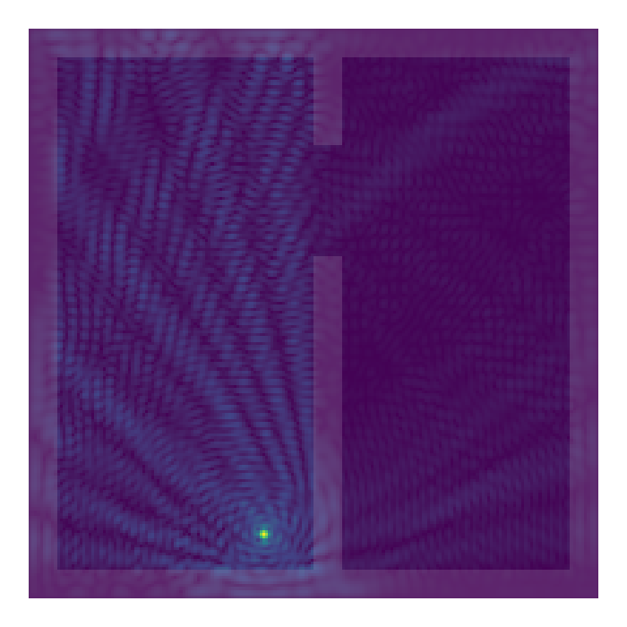
Nice. The signal gets weaker the further away we move from the source. We get reflection on the walls due to the refractive index greater than one. We also get damping of waves that penetrate the walls due to the positive damping term. And since the walls aren't perfect insulators, some of the waves that penetrate make it through the walls to propagate into the neighboring room.
The code takes around 5 seconds for a 200 by 200 grid, which is acceptable, but can probably be improved by better exploiting the structure of the linear operator. Since the sparse solver from the Matrix package uses optimised C code, I don't expect any speed up from coding this up in python or another language.
Could this simulation really be used to optimise placement of the wifi router for best coverage, given the floor plan of an appartment? I don't know. First I would probably study the sensitivity of the simulation to the refraction and damping parameters. There seem to be numerical artifacts due to the coarse spatial resolution. The fact that I'm essentially setting zero boundary conditions outside the outer walls is also problematic. I'm also wondering how such a model could be calibrated on real data. But all of that is for another day. For today I'm happy that my code generated results that look halfway reasonable.
Varying the refractive index of the walls
Varying the damping coefficient
Varying position