set.seed(1)
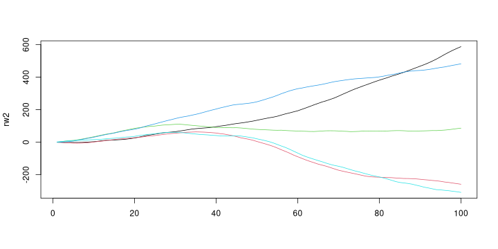
rw2 = sapply(1:5, function(ii) cumsum(cumsum(rnorm(100))))
matplot(rw2, type='l', lty=1)

The 2nd order random walk (RW2) is a time series model defined by \[x_t = 2 x_{t-1} - x_{t-2} + \epsilon_t\] where \(\epsilon_t \sim N(0,\tau_x^{-1})\) is iid Normal with precision \(\tau_x\).
The RW2 is a popular prior for temporally correlated data used in time series modelling and Bayesian hierarchical modelling.
Realisations of the RW2 can be generated by realising that the second-order differences \((x_t - x_{t-1}) - (x_{t-1} - x_{t-2})\) are iid Normally distributed. The inverse operation of differencing is the cumulative sum, so one way to generate realisations of RW2 is to cum-summing iid Normal random variables twice.
set.seed(1) rw2 = sapply(1:5, function(ii) cumsum(cumsum(rnorm(100)))) matplot(rw2, type='l', lty=1)

If the vector \(x = (x_1, x_2, \dots, x_n)\) is a realisation of RW2, we can show that \(x\) has a multivariate Normal distribution. The likelihood of \(x_3, \dots, x_n\), is given by \[\begin{aligned} \log p(x_3, \dots, x_n | x_1, x_2) & = \sum_{t=3}^n \log p(x_t|x_{t-1}, x_{t-2}, \tau_x)\\ & = const - \frac{\tau_x}{2} \sum_{t=3}^n (x_t - 2 x_{t-1} + x_{t-2})^2 \end{aligned}\] The sum of squares can be written as the dot product of a vector \(z\) with itself, where here \(z\) is given by \[z = D x = \begin{pmatrix}1 & -2 & 1\\& \ddots & \ddots & \ddots\end{pmatrix} x\] Here \(z\) has length \(n-2\) and \(D\) has \(n-2\) rows and \(n\) columns. Plugging this into the likelihood, we have \[\begin{aligned} \log p(x_3, \dots, x_n | x_1, x_2) & = \sum_{t=3}^n \log p(x_t|x_{t-1}, x_{t-2}, \tau_x)\\ & = const - \frac{1}{2} x'(\tau_x D'D)x\\ & = const - \frac{1}{2} x' Q_x x \end{aligned}\] Assuming that \(x_1\) and \(x_2\) have a joint uniform prior distribution, i.e. \(p(x_1, x_2| \tau_x) = const\), the full joint distribution of the vector \(x\) is that of a multivariate Normal distribution \[\begin{aligned} p(x|\tau_x) & = p(x_1, x_2 | \tau_x) \prod_{t=3}^n p(x_t|x_{t-1}, x_{t-2}, \tau_x)\\ & = const \times e^{-\frac12 x' Q_x x} \end{aligned}\] with precision (inverse variance) matrix given by \[Q_x = \tau_x D'D = \tau_x \begin{pmatrix} 1 & -2 & 1\\ -2 & 5 & -4 & 1 \\ 1 & -4 & 6 & -4 & 1\\ & \ddots & \ddots & \ddots & \ddots & \ddots\\ && 1 & -4 & 6 & -4 & 1\\ &&& 1 & -4 & 5 & -2\\ &&&&1 & -2 & 1 \end{pmatrix}\]
Let's first assume that \(\tau_e\) and \(\tau_x\) are known. How do we infer the latent vector \(x\) from the observed data \(y\)?
The joint log-density of \(x\) and \(y\) is given by \[\begin{aligned} \log p(x,y) & = \log p(y|x) + \log p(x)\\ & = const - \frac12 (y - x)'Q_e (y - x) - \frac12 x' Q_x x \end{aligned}\] We want to infer \(x\) from \(y\), that is we want to calculate \(p(x|y)\): \[\begin{aligned} \log p(x|y) & = const + \log p(x, y)\\ & = const - \frac12 x'(Q_x + Q_e)x + (Q_e y)'x\\ \end{aligned}\] This is the density of the multivariate Normal distribution in canonical form, and so the conditional distribution of \(x\) given \(y\) is multivariate Normal with conditional expectation \[E(x|y) = (Q_x + Q_e)^{-1}Q_e y\] and conditional variance \[Var(x|y) = (Q_x + Q_e)^{-1}.\]
library(tidyverse)
library(Matrix)
# simulate latent x, errors, and observations
set.seed(18)
n = 50
tau_x = 10
tau_e = 0.1

xy = tibble(t=1:n,
            x=cumsum(cumsum(rnorm(n, 0, 1/sqrt(tau_x)))),
            y=x + rnorm(n, 0, 1/sqrt(tau_e)))

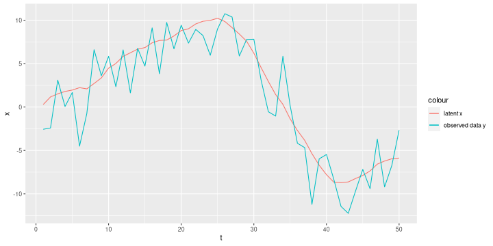
ggplot(xy, aes(x=t)) +
  geom_line(aes(y=x, colour='latent x')) +
  geom_line(aes(y=y, colour='observed data y'))

# define precision matrices Q_e and Q_x
Qe = tau_e * Diagonal(n)
Dx = bandSparse(n=n-2, m=n, k=0:2,
                diagonal=list(rep(1, n-2), rep(-2, n-2), rep(1, n-2)))
Qx = tau_x * crossprod(Dx)
y = xy$y

# calculate conditional expectation and marginal variances
mu_x = drop(solve(Qx + Qe, Qe %*% y))
sigma_x = sqrt(diag(solve(Qx + Qe)))

xy = xy %>% mutate(mu_x = mu_x, sigma_x = sigma_x)

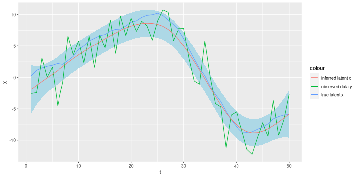
ggplot(xy, aes(x=t)) +
  geom_ribbon(aes(ymin=mu_x - 2 * sigma_x,
                  ymax = mu_x + 2 * sigma_x),
        fill='lightblue') +
  geom_line(aes(y=x, colour='true latent x')) +
  geom_line(aes(y=y, colour='observed data y')) +
  geom_line(aes(y=mu_x, colour='inferred latent x'))

So far we have assumed that the hyperparameters \(\tau_x\) and \(\tau_e\) are known. In practice it's rare that we know the variances of the latent process or the measurement error, so we might want to estimate them.
The following approach calculates the posterior of the hyperparameters \(\theta = (\tau_x, \tau_e)\) given the observed data \(y\). It uses the two alternative factorisations of the joint density distribution \[ p(y,x,\theta) = p(y|x,\theta)p(x|\theta)p(\theta) = p(x|y,\theta)p(y|\theta)p(\theta)\] and solves for \(p(\theta|y)\) treating all functions that don't depend on \(\theta\) as a multiplicative constant \[\begin{aligned} p(\theta | y) & = \frac{p(x,y,\theta)}{p(x|y,\theta)p(y)}\\ & = const \times \frac{p(y|x,\theta)p(x|\theta)p(\theta)}{p(x|y, \theta)} \end{aligned}\]
One source of confusion is the occurrence of \(x\) on the rhs but not on the lhs, so we might ask, what configuration of \(x\) do we use on the rhs? The answer is, any configuration for which \(p(x|y,\theta)\) is non-zero. The conditional expectation \(x^* = E(x|y,\theta) = (Q_x + Q_e)^{-1}Q_e y\) is a natural choice.